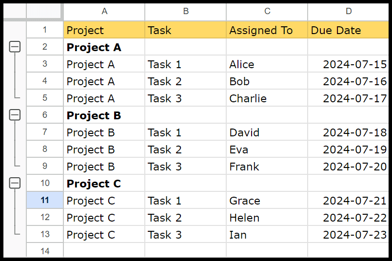
Let’s say you are managing a list of tasks for your team in Google Sheets and want to organize these tasks by project. Each project has several tasks listed one after another.
By grouping rows for each project, you can make your sheet easier to read and use. This way, you can collapse and expand the project tasks, making the sheet cleaner and more organized.
By grouping rows for the projects, you can collapse sections you don’t need to see all the time.
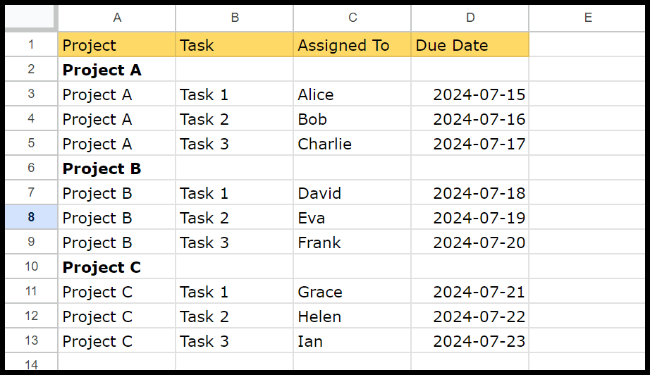
In the data above, we have three tasks for each project, and there is a blank row with the project’s name above each product. This blank row is a title when you group rows and then collapse the group.
Simple Steps-by-Step Guide to Group Rows in Google Sheets
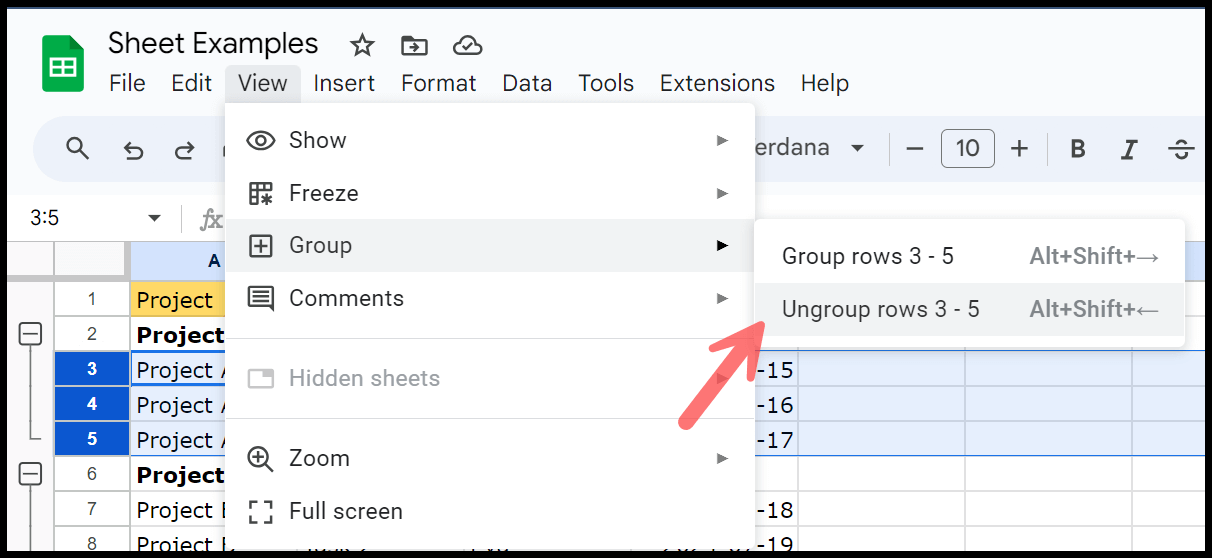
Grouping rows in Google Sheets is quite simple and quick; you only need to select the rows and use the option from the View > Group > Group Rows, or you can use the keyboard shortcut Alt + Shift + Right Arrow.
And if you want to see how I have done it for the data I have in my sheet, you can use the below steps:
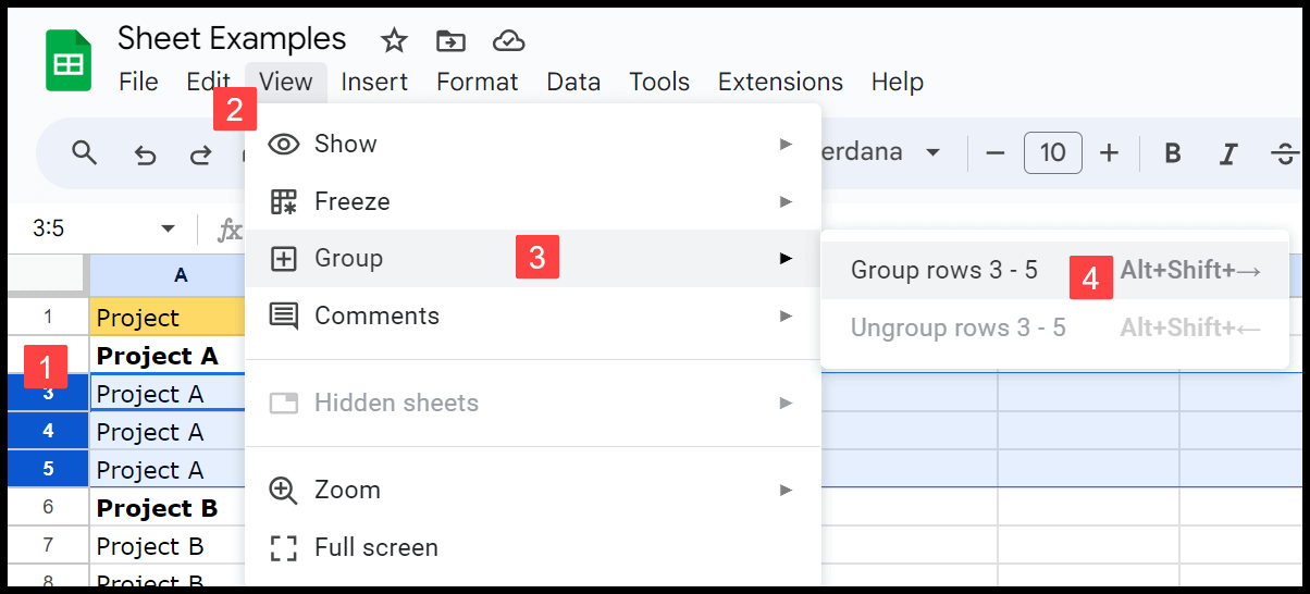
- First, select the rows you want to group. For “Project A,” select rows 3 to 5.
- After that, go to the “View” menu on the menu bar and click on the “Group” option.
- Now, you will have further options in the “Group” option.
- From there, select “Group rows 3 – 5” to group the selected rows (3-5).
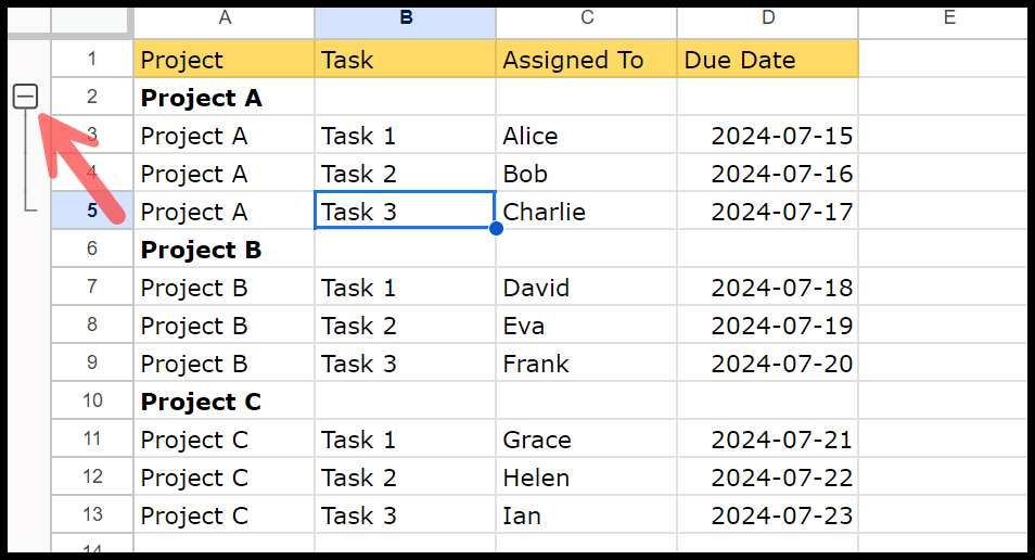
Selecting the option groups all the rows and gives you an expand and collapse button on the row above the selected rows.
Read Also – Unhide Rows in Google Sheets
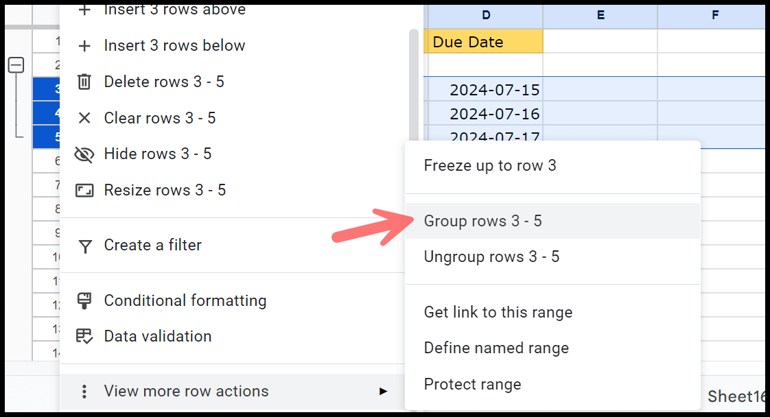
Instead of the Edit menu, you can right-click after selecting the rows, go to the “View more rows action”, and then go to the “Group rows 3 -5”.
Repeat the process for the other projects. For “Project B,” select rows 7 to 9 and group them. For “Project C,” select rows 11 to 13 and group them. Each group will have a small minus sign to click to collapse or expand the tasks.
Read Also – Remove Blank Rows in Google Sheets
How to Ungroup Rows in Google Sheets
Ungrouping rows is just as simple as grouping them. Here’s how you can do it in a few easy steps:
- First, select the rows you want to ungroup. Click on the small plus sign on the left side of the grouped rows to expand them. Then, select all the rows within the group.
- Once the rows are selected, click “View,” then choose “Ungroup rows.” It will remove the grouping, and the minus and + sign will disappear from the left side of the rows.
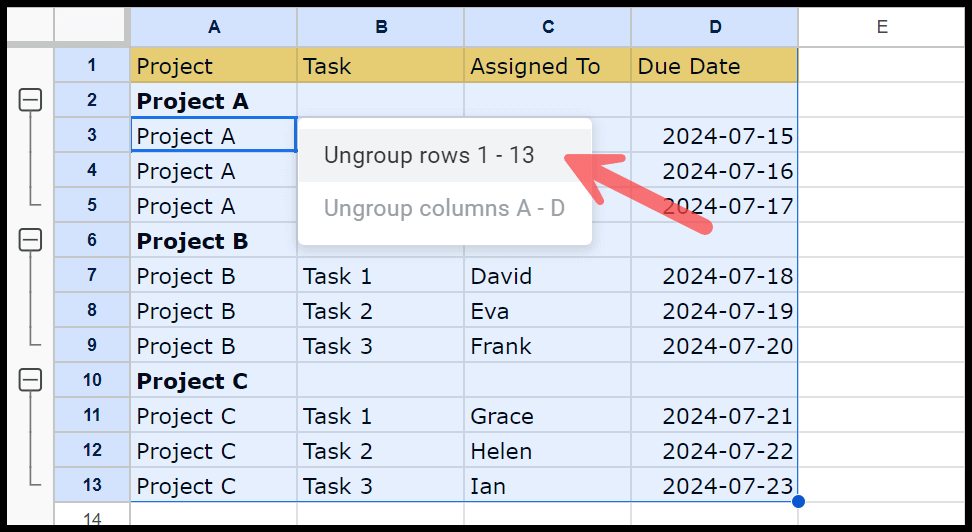
Repeat this for all the other groups of rows that you have in the worksheet. If you want to remove all the groups of rows in the worksheet in one go, you can use the below steps:
Select the entire data with the keyboard shortcut Ctrl + A, and then use the keyboard shortcut Shift + Alt + Left Arrow; this will show you a pop-up menu and then
Read Also – Delete Rows in Google Sheets
Quick Tip: When creating reports, use row grouping to create collapsible sections. This allows viewers to expand sections for detailed information and collapse them for a summary view.
Grouping Options
When you right-click on the Expand-Collapse button, a small menu with a few options appears.
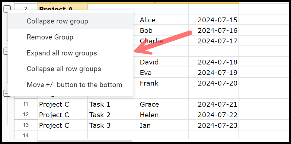
Two options are unique from this list and have not been listed anywhere else. The first is to collapse and expand all the row groups, and the second is to move the buttons to the bottom of the group.
Note: When you copy and paste data from a row with a group, that group doesn’t get moved with the data.
Group and Ungroup Columns in Google Sheets
Grouping and Ungrouping columns is like grouping rows in Google Sheets. To group and ungroup columns manually, follow these steps:
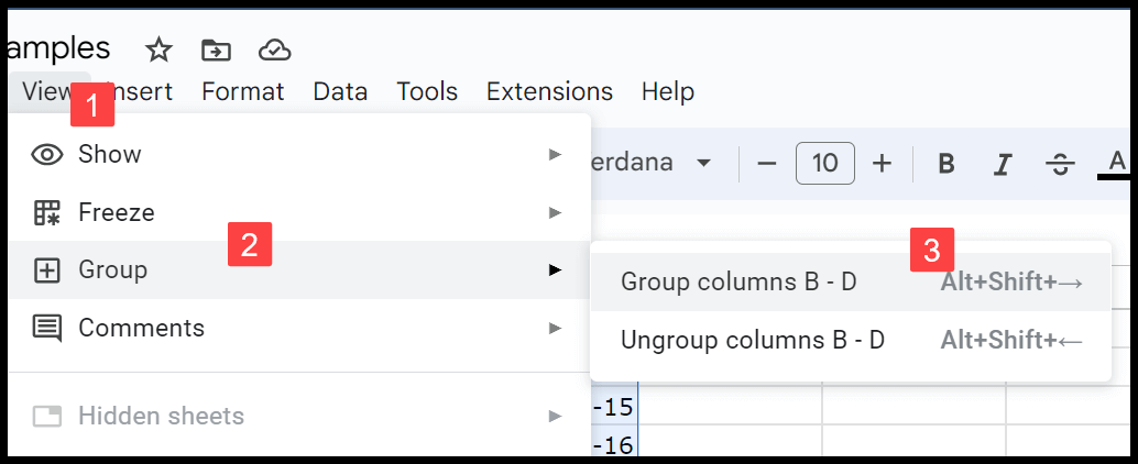
- Select the columns you want to group. For example, select columns B to D using your mouse to group columns B to D.
- Go to the ribbon at the top of the screen, click View, and click “Group columns B-D”. A small minus sign will appear above the grouped columns, indicating they are now grouped.
Or you can use the keyboard shortcut Shift + Alt + Right Arrow. You can use the same steps to ungroup columns or the keyboard shortcut Shift + Alt + Left Arrow.