How to use VLOOKUP MATCH Combination in Excel (Formula)

The Combo of VLOOKUP and MATCH is like a superpower. Well, as we all know VLOOKUP is one of the most popular functions.

Right?

It can help you quickly lookup a value in a column. But when you use it more and more you will realize some problems with it. And, the biggest problem is it’s not dynamic.

In VLOOKUP, col_index_no is a static value which is the reason VLOOKUP doesn’t work as a dynamic function. And this is where you need to combine VLOOKUP with MATCH. 

If you are working on multiple-column data, it’s a pain to change its reference you have to do (change the column number) manually.

The best way to solve this problem is to use the MATCH function in VLOOKUP for col_index_number. Today in this post, I going to explain all the stuff you need to know to use this combo formula.

Problems With VLOOKUP

I have found the two biggest reasons to create a combination of these two functions.

1. Static Reference

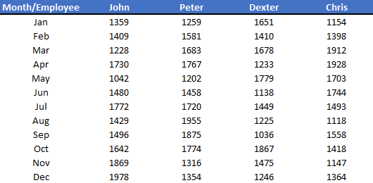
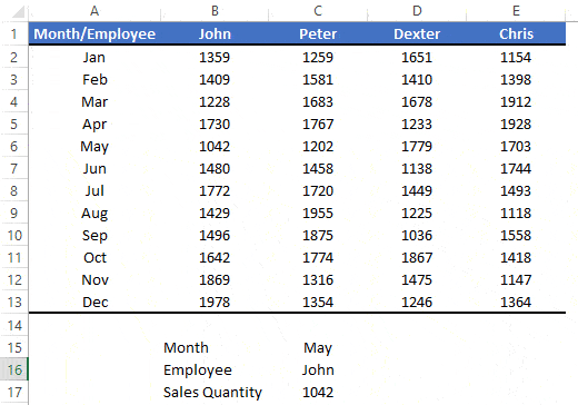
Just look at the below data table where you have 12-month sales for four different employees.

Now, let’s say you want to look up the Feb month’s sale of “John”. The formula should be like this.

=VLOOKUP("May",A1:E13,2,0)

In this formula, you have mentioned 2 as the col_index_num because John’s sale is in the second column. But what will you do if your boss tells you to get the sales value for “Peter”?

You need to change the value in col_index_num because it’s not dynamic.

2. Add or Delete Columns

Now think in a different way. You need to add a new column for a new employee just before John’s column.

And here, John’s column number is 3 and your formula result is incorrect.

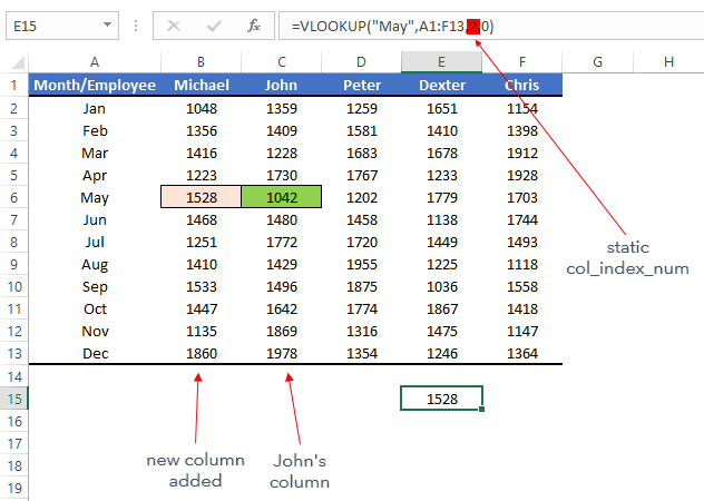
Again here, because col_index_num is a static value you need to change it manually from 2 to 3 and again if you need something else.

At this point, you are clear about one thing you need to make col_index_num dynamic. And for this, the best way is to replace it with the MATCH function.

Why Match Function

Before you combine VLOOKUP and MATCH, you need to understand the match function and its work. The basic use of MATCH is to find the cell number of the lookup value from a range.

Syntax: MATCH(lookup_value,lookup_array,[match_type])

It has mainly three arguments, lookup value, a range to lookup for the value, and the match type to specify an exact match or an approximate match.

For example, in the below data, I am lookup for the name “John” with the match function from a heading row.

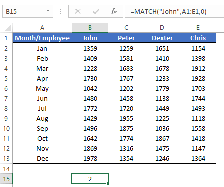
And, it has returned 2 in the result because the name is in the 2nd cell of the row.

VLOOKUP and MATCH Together

Now, it’s time to put VLOOKUP and MATCH together. So, let’s continue with our previous example.

First of all, let’s create a formula by using both of the functions, and then we’ll understand how these two work together.

Steps to create this combo formula:

• First of all, in one cell enter the month’s name, and in another cell enter the employee’s name.
• After that, enter the below formula in the third cell.

=VLOOKUP(C15,A1:E13,MATCH(C16,A1:E1,0),0)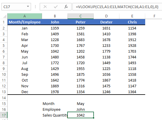

In the above formula, you have used VLOOKUP to lookup for the MAY month, and for the col_index_num argument, you have used the match function instead of a static value.

And in the match function, you have used “John” (employee name) for the lookup value.

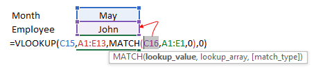
Here match function has returned the cell number for the “John” from the above row. After that, VLOOKUP used that cell number to return the value.

In simple words, the MATCH function tells VLOOKUP the column number to get the value from.

Problems Solved?

Above you have learned about two different problems which are because of static col_index_num.

And, for this, you have combined VLOOKUP and MATCH. Now, we need to check whether those problems are solved or not.

1. Static Reference

You have referred to the employee name in the match function to get the column number for VLOOKUP.

When you change the employee name in the cell, the match function will change the column number. And when you need to get the value for a different employee you have to change the employee name in the cell.

This way, you have a dynamic col_index_number.

Finally, you don’t have to edit the formula again and again.

2. Add or Delete Columns

Before adding a new column John’s data was in the 2nd column and the match function returned 2. And after you have inserted a new column john’s data is in the 3rd column and the match returned 3.

When you add a new column for a new employee the value in the formula is not changed because the match function updates its value.

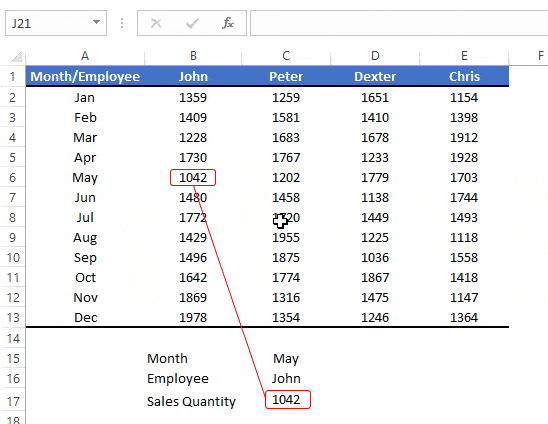
In this way, you’ll always get the correct column number even when you insert/delete any column. The MATCH function will return the right column number.