Lookup Last Value from a Column or a Row in Excel (Formula)

In Excel, there are two ways to look for a value from a column or a row. In this tutorial, we will learn to use both formula types and try to cover them in different situations.

Lookup the Last Value (When the Last Value is in the Last Cell)

Follow these steps to write this formula:

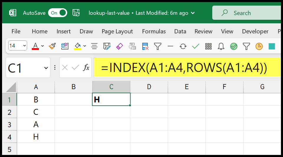
1. First, enter the INDEX function in a cell.
2. After that, in the array argument, refer to the range of values.
3. Next, in the rows argument, enter the ROWS function.
4. In the ROWS function, refer to the range where you have values.
5. In the end, enter the closing parentheses and hit enter to get the result.

=INDEX(A1:A4,ROWS(A1:A4))

The moment you hit enter, it returns the value from the last cell of the range.

The only problem with this formula is when you don’t have a value in the last cell of the range.

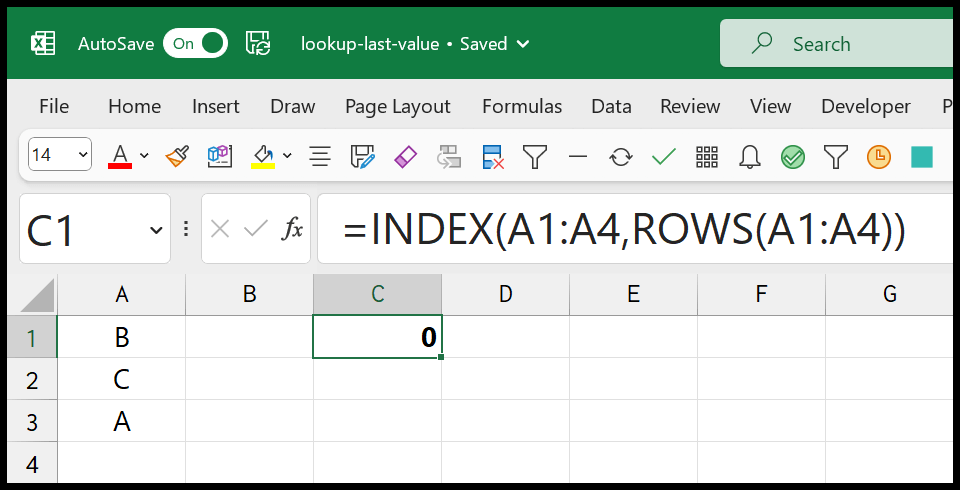
Therefore, we can switch to the formula we will discuss next.

Lookup Last Value in Column

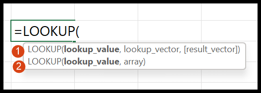
You can use the LOOKUP function also. And the formula will be:

=LOOKUP(2,1/(A:A<>""),A:A)

LOOKUP has two syntaxes to follow, and we have used the vector syntax.

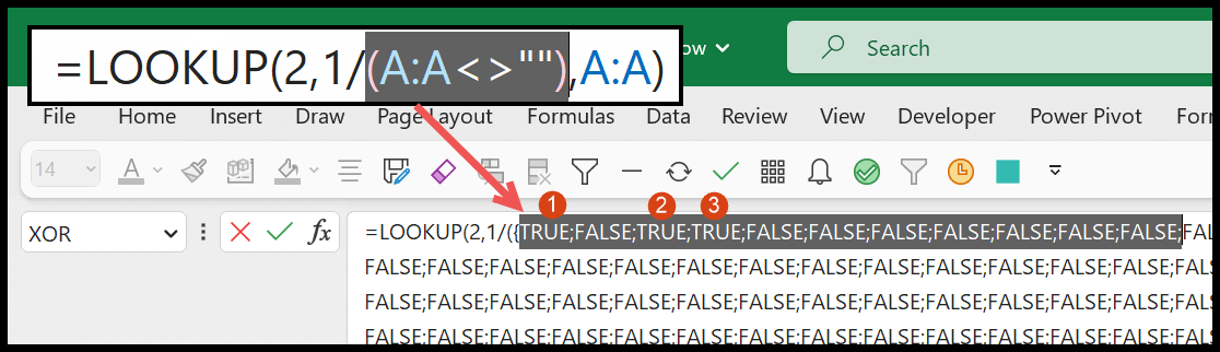
(A:A<>””)

This part of the formula returns an array after testing whether a cell has a value.

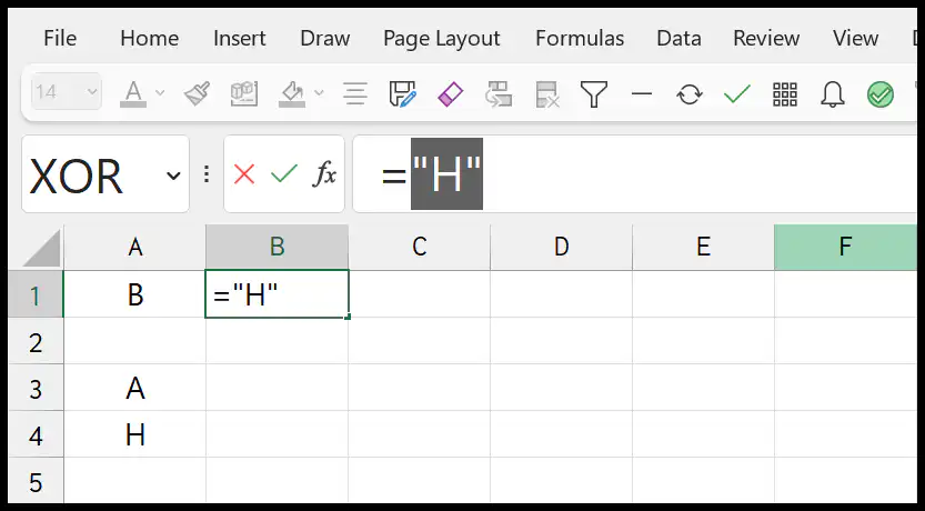
Here we have referred to the entire column, and that’s why it has returned a large array. But in the first three values, you can see we have TRUE, which is because we have the values in the first three cells in column A

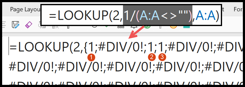
1/(A:A<>””)

And when you divide 1 with the entire array returned by the earlier part of the formula, you get 1 for TRUE and;#DIV/0! for all the FALSE values.

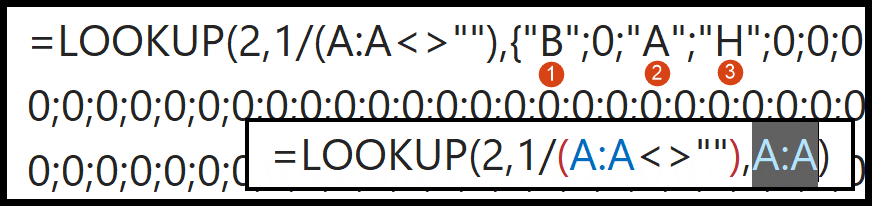
A:A

In this part of the formula, you have the reference to column A. And it returns an entire array of values from the column. Where the cell is blank, you have a 0, and the actual value where the cell is not blank.

LOOKUP(2,1/(A:A<>””),A:A)

As I mentioned earlier, we used the LOOKUP function’s vector syntax.

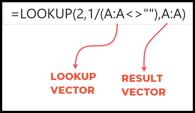
• In the LOOKUP vector, we have all the values as 1 and 0. 1 where we have the values in the RESULT vector, and 0 where we don’t have any value in the result vector.
• When you lookup for 2 in the range where you have 1 in all the values, the LOOKUP function will refer to the last 1 in the LOOKUP vector.
• Then it returns the corresponding value from the result vector. That last value is the exact last value in column A.

Lookup for the Last Value from a Row

It can be used to get the value from the last non-empty cell from a row. So you only need to change the reference that you have.

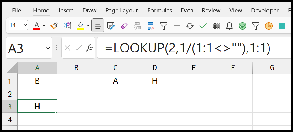
=LOOKUP(2,1/(1:1<>""),1:1)

In this formula, we have referred to the entire row (Row 1) for the lookup vector and in same in the result vector. And when you hit enter, it returns the value from cell D1 which is the last non-empty cell in the row.