Randomize a List (Shuffle Data using Random Sort) in Excel

To randomize the list of values in Excel means you can randomly sort data. And for this, you need to use Excel’s RAND function and along with that, you need to use the sort feature that you use to sort data. RAND gives random values that help to shuffle that data randomly.

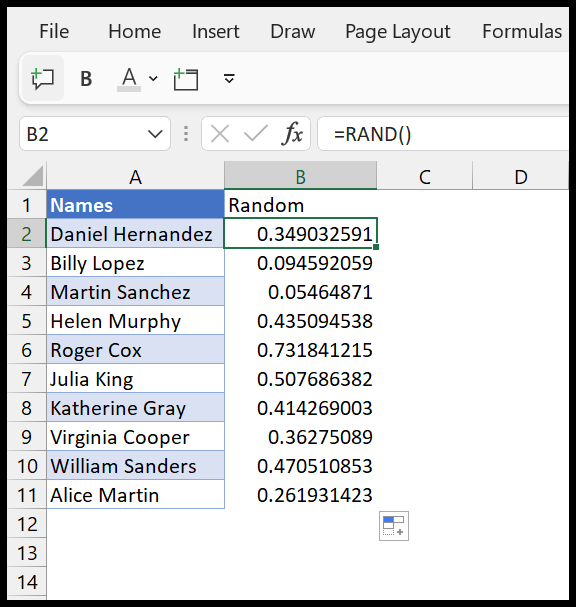
In the following example, we have a list of names and now we need to sort this list using a random order.

Steps to Random Sort a List in Excel (Randomize a List)

1. First, enter RAND() in cell B1. This will give you a random number between 0 and 1.
2. Next, you need to drag the formula up to the last name that you have in the list.
   
3. From here you need to open the sort option from the DATA ➜ SORT. Or you can use the keyboard shortcut (Alt ➜ A ➜ S ➜ S).
   
4. In the “Sort by” select the name of the column where you have random values and select the order you want (this doesn’t make any difference because we are looking for random sorting).
5. In the end, click OK.

And once you click OK, you have a randomized list of names (sorted by random order).

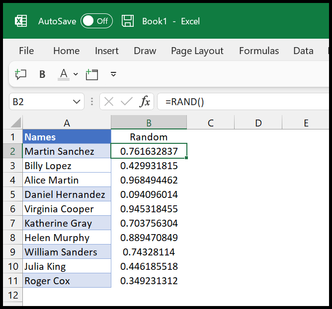
Now there’s one thing that we need to note down here. The RAND function is a volatile function and it changes every time you re-calculate in Excel. Either you can change those random values into actual values, or if you want to re-sort names you can leave it the way it is.

Random Sort Columns

You can also sort columns in a random order using the same method. In the following example, we have the same list of names in multiple columns and now we need to sort columns in random order.

First, you need to create a random number column the way we have done in the previous method.

After that, you need to select the data range from both rows.

Now the next thing that we do is to open the sort option. And in the sort option, click on the “OPTIONS” button and select the “SORT LEFT TO RIGHT” option, and then click OK.

Now in the sort options dialog box, select “Row1” and at the end, click OK.

And the moment you click OK, you’ll get the columns sorted in random order.

So, this is how you can use randomize a list of values in Excel using a random sort method.