How to Calculate Mean in Excel

One of the best things about Excel is that you can use formulas and functions to calculate different statistical terms like mean, mode, and median. In today’s tutorial, I will share with you how to calculate the mean in Excel using various formulas, and we will discuss how these formulas work in detail.

Key Points

• There are two major ways to calculate the mean. One uses the AVERAGE Function, and the second uses a formula based on SUM and COUNT.
• You can also create a custom function using a VBA code and use TRIMMEAN to calculate the mean by ignoring outliers.

What is a Mean?

In simple math and statistical calculations, the mean is the average value of a set of numeric values. It is calculated by adding all the numbers together and then dividing that sum by the total number of numbers. When it comes to Excel, as I said, there are multiple ways that you can use to calculate the mean.

Also, the mean is a calculation of central tendency, which essentially refers to a value representing the center of a set of numbers. In the context of a statistical distribution, the mean is used to describe the location of this central point.

Calculate MEAN with the AVERAGE Function in Excel

AVERAGE is the perfect function for getting the mean from numbers. The numbers below are in the range A1:A11. Now, we need to calculate the mean in cell B1.

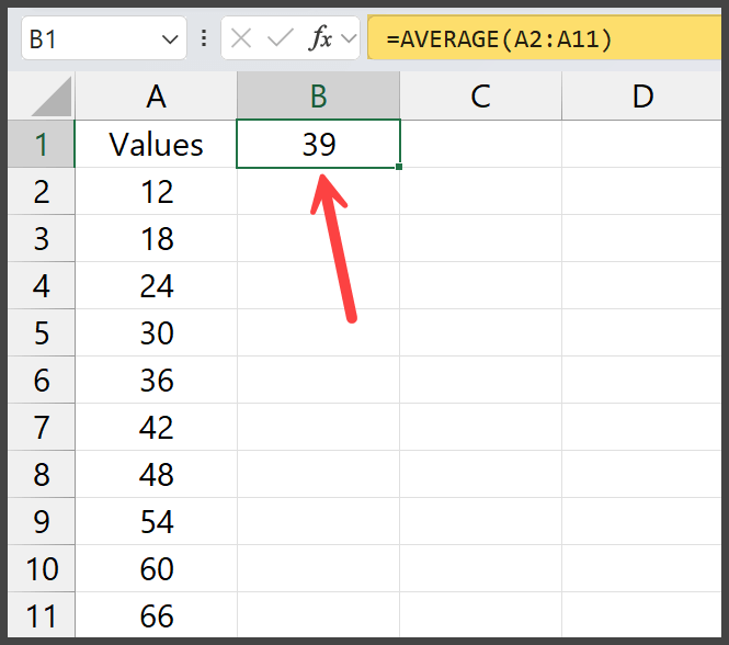
Here are the steps to calculate the mean:

1. Enter the =AVERAGE( in the cell B1.
2. Refer to the range A2:A11.
3. Close the function by entering the “0”.
4. Hit enter to get the mean in the result.

In the same way, if you have data in different ranges, you can refer to those ranges in the function just by using the (,) to refer to multiple ranges.

Sometimes, the mean may result in decimal places. Consider rounding using =ROUND(AVERAGE(range),0) if you need a whole number.

Let’s say you have values in the range A2:A1 and B2:B11. You can use a formula like the following:

=AVERAGE(A2:A11,B2:B11)

Excel’s AVERAGE function is easy to use, but you must consider the data you refer to in the formula.

You need to understand that Excel users have a misconception about BOOLEAN values in the data while using the AVERAGE. But the truth is that using the “AVERAGE” function won’t consider the TRUE and FALSE while returning the result.

Let’s take an example where you have an error value in the data. The AVERAGE function will return an error in the result, as shown in the example below.

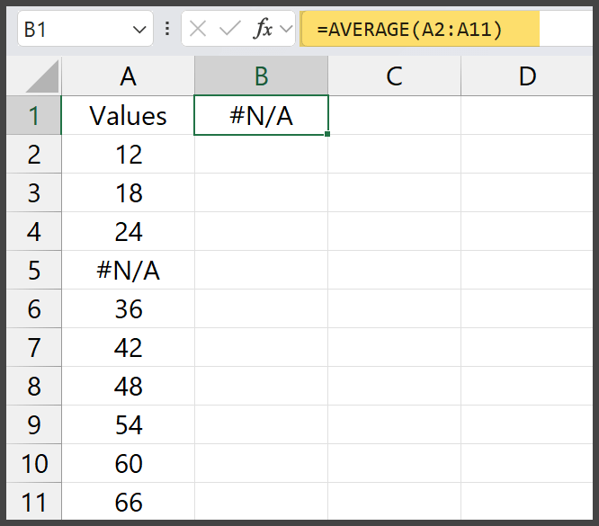
In cell A5, we have an #N/A error, and that’s why we have the same error in the result. But here’s the happy news: we have a solution to this problem.

All you need to do is to use the AVEARGEIF function instead of the AVERAGE. Here’s the formula:

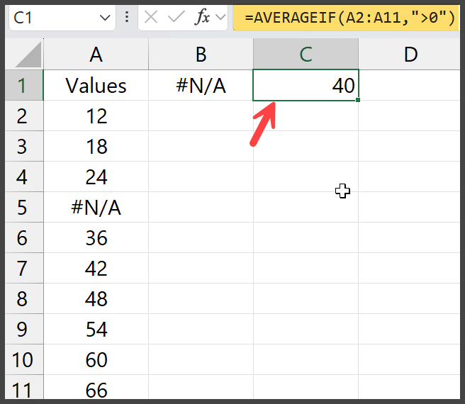
=AVERAGEIF(A2:A11,">0")

This formula allows you to calculate the mean of numbers based on a condition.

In this case, the condition is that the values must be greater than 0, meaning that only valid numeric values are included, and the #N/A error is ignored.

This formula works for all the errors while calculating the mean as it ignores the #N/A and focuses on the valid numeric values greater than 0 (12, 18, 24, 36, 42, 48, 54, 60, 66).

The sum of the valid numbers is 360, with 9 numbers, so the average is calculated as 360 / 9 = 40.

Read Also – Calculate MEDIAN IF in Excel / Calculate T-Test (T.Test) Google Sheets / Average Numbers but Exclude Zeros

Combine SUM And COUNT to Get Mean for Values

If you don’t want to use the AVERAGE function, which is one of the best ways to get the mean of a number, you can create a custom formula by combining SUM and COUNT.

Below is the formula that you can use:

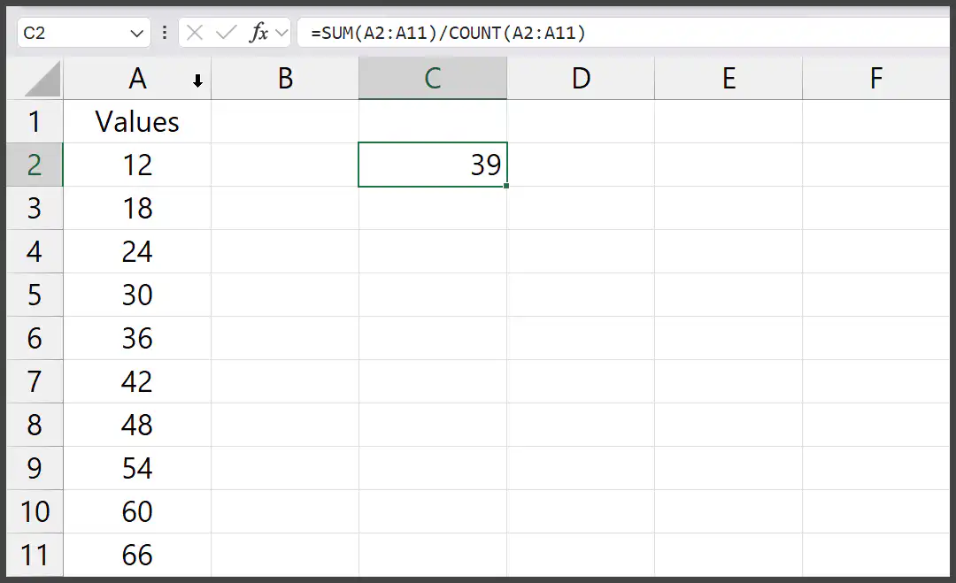
=SUM(A2:A11)/COUNT(A2:A11)

To understand this formula, you need to split it into parts. Here’s how this formula works:

• SUM(A2:A11) – In the first part, we have an SUM function that calculates the total values from A2 to A11. In this case, it adds up to 12, 18, 24, 30, 36, 42, 48, 54, 60, and 66.
• COUNT(A2:A11) – In the second part, the COUNT function counts the number of numeric values in the range A2 to A11. Since there are 10 numbers in this range, the result is 10.
• / – In the third part, the formula divides the sum of the values by the count of the values to get the mean.

The sum of the numbers is 390, and since there are 10 numbers, the average is calculated as 390 / 10 = 39, which is the value we have in cell C2.

Custom VBA Function to Calculate the Mean in Excel

Both methods are impressive, but if you want a custom function to calculate the mean in Excel, which can take care of blank cells and errors, and an option to ignore zeros, you can use the code below.

This code creates a custom function that can add a function in Excel that you can use.

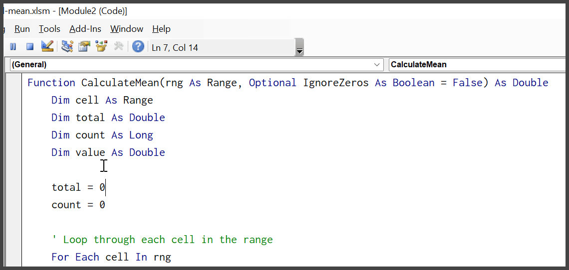
Function CalculateMean(rng As Range, Optional IgnoreZeros As Boolean = False) As Double
    Dim cell As Range
    Dim total As Double
    Dim count As Long
    Dim value As Double
    total = 0
    count = 0
    ' Loop through each cell in the range
    For Each cell In rng
        ' Check if the cell contains a number and is not blank or an error
        If IsNumeric(cell.Value) And Not IsEmpty(cell.Value) Then
            value = cell.Value
            ' Check if the user wants to ignore zeros and if the value is not zero
            If IgnoreZeros = True Then
                If value <> 0 Then
                    total = total + value
                    count = count + 1
                End If
            Else
                total = total + value
                count = count + 1
            End If
        End If
    Next cell
    ' Check to avoid division by zero
    If count > 0 Then
        CalculateMean = total / count
    Else
        CalculateMean = 0 ' Return 0 if no valid numbers were found
    End If
End Function

Read Also – Personal Macro Workbook / Custom Function in Excel

• To use this code, first open the Excel workbook, press Alt + F11 to open the VBA editor, go to Insert > Module, and paste the code there.
• Close the VBA editor.
• Now, in any cell in the worksheet, you can use the CalculateMean function like a normal Excel function.

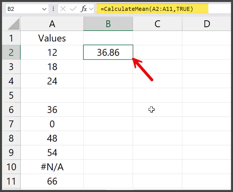
To calculate the mean of a range (e.g., A1:A10), type =CalculateMean(A1:A10). To calculate the meanwhile ignoring zeros, type =CalculateMean(A1:A10, TRUE).

How does this code work to create this custom function?

This code creates a custom function, CalculateMean, which calculates the average of a range of cells while ignoring blank cells and cells with errors. It loops through each cell in the specified range and checks if the value is a number. If it is, it adds that value to the total and counts it.

It also has an optional argument, IgnoreZeros. If set to True, the function will skip any zeros in the range. After going through all the cells, the code divides the total by the number of valid values to return the mean or returns zero if no valid values are found.

Using the TRIMMEAN Function to Calculate the After Excluding the Outliers

With the TRIMMEAN, you can calculate the mean of a set of values while excluding a specified percentage of outliers from the data’s top and bottom.

This is useful when removing extreme values that may affect the average.

=TRIMMEAN(array, percent)

In the percent argument, using 0.2 specifies 20%, which means 20% of the values (10% from the highest and 10% from the lowest) will be ignored.

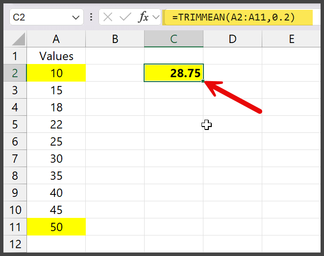
This will exclude the top 10% (one value from the highest end) and the bottom 10% (one from the lowest end), leaving the middle eight values to calculate the mean.

The mean will be based on the numbers 15, 18, 22, 25, 30, 35, 40, 45. If you calculate the mean for all the values, it comes to 29.5, but when you calculate using the TRIMMEAN, it comes to 28.75.

It provides a more robust mean by ignoring extreme values that may distort the average.

Excel ignores text values in a numeric range, so ensure no number stored as a text is present, as it could effect your results.