

Open both workbooks, type = in the destination cell, switch to the other workbook, click the source cell and press Enter. Excel writes the link for you, for example =[Book2.xlsx]Sheet1!$A$1, and the cell shows the source value.
To type the link yourself, put the workbook name in square brackets, then the sheet name and !: =[Book2.xlsx]Sheet1!A1. If either name contains a space, wrap both in apostrophes: ='[Sales Data.xlsx]Jan Sales'!A1. When the source is closed, add the folder path inside the apostrophes: ='C:\Reports\[Sales Data.xlsx]Jan Sales'!A1.
To link a whole block at once, copy the source range, go to the destination and choose Home → Paste → Paste Link, or right-click and use Paste Special → Paste Link. To open another file from a cell rather than pull its values, press Ctrl + K and choose Existing File or Web Page.
The click method inserts an absolute reference such as $A$1, so every copy points at the same source cell when you fill the formula down or across. Delete the $ signs before you copy it.
Links break when the source file is renamed or moved, and SUMIF, COUNTIF and INDIRECT return #VALUE! or #REF! while the source workbook is closed. Use Data → Workbook Links (Data → Edit Links in older versions) to update, change the source or break links, and click Enable Content when Excel blocks the update on opening.
Excel has multiple ways to create a link between two workbooks.
- Referring to a Range with Click
- Copy and Paste the Range Address
- Use the Hyperlink Option
- Manually Write a Formula or a Reference
In this tutorial, we will learn all these methods in detail. So, let’s get started:
Referring to a Range with Click
- First, open both workbooks.
- Select a cell in the workbook in which you want to create the link and type an equal sign (=).
- Now, go to the other workbook, select the worksheet and click on a cell.
- In the end, press Enter. Excel takes you back to the first workbook and shows the value from the other workbook in the cell.
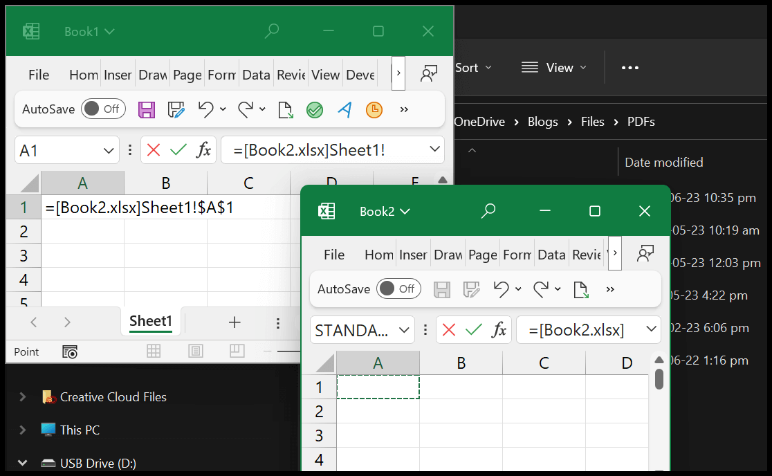
Once you press Enter, the cell holds a formula like the one below. It has the workbook’s name in square brackets, the sheet’s name, an exclamation mark and the cell address:
=[Book2.xlsx]Sheet1!$A$1
You can use the same method inside a function. Type the function name and the opening parenthesis (for example, =SUM( ), then go to the other workbook, select the range and press Enter:
=SUM([Book2.xlsx]Sheet1!$A$1:$A$10)
Paste the Link to Another Workbook
Another method is to copy a cell from the source workbook (the one you want to link to) and paste it as a link in the workbook where you want to create the link.

- First, open both workbooks and copy a cell (Ctrl + C) from the workbook you want to link to.
- Afterwards, go to the workbook where you want to create the link and select a cell.
- Now, right-click and then click on “Paste Special”.
- Finally, click on “Paste Link” to create a link to that cell.
You can also use the ribbon for this: Home > Paste > Paste Link. And if you copy more than one cell, Excel creates a link for each cell you paste, so you can link a whole table in one go.
The values you paste this way update when the values in the source workbook change.
Use the Hyperlink Option to Link to Another Workbook
And you can also create a direct hyperlink to a workbook. For this, you need to use the hyperlink option.
Note: For this method, you don’t need to open the workbook for which you want to create the link.
First, select the cell where you want the link. After that, right-click > Link > Insert Link.

Or you can go to the Insert tab > Link > Insert Link. You can also press Ctrl + K (Command + K on a Mac) to open the same dialog box.

This will open a dialog box to insert a hyperlink. In this dialog box, you need to click on “Existing File or Web Page” and locate the workbook for which you want to create a hyperlink.

Once you locate it, select the file and click OK. Once you click OK, it creates a link to book2 (another workbook) with the workbook’s name in your selected cell.

Keep in mind that a hyperlink only opens the other workbook when you click on it. It doesn’t bring any values from that workbook into your cell. To jump to a specific cell, click the Bookmark button in the same dialog box and pick the sheet and the cell.
You can also create the same link with the HYPERLINK function. In the first argument, enter the file path and the workbook’s name in square brackets, followed by the sheet and the cell, and in the second argument, the text you want to show in the cell:
=HYPERLINK("[C:\Reports\Book2.xlsx]Sheet1!A1","Go to Book2")
Write a Reference in a Formula
You can also write a reference manually by typing it in the cell. Let’s say you want to refer to book2. There are two ways to do that:
1. When Workbook is Open
When the workbook you want to link to is open, you need to use the name of the workbook, the sheet’s name, and then the cell or range address.

- First, type an equal sign.
- Then, enter the workbook’s name with the file extension and wrap it in square brackets.
- After that, enter the sheet’s name, followed by the exclamation mark.
- In the end, enter the address of the cell or the range.
Here’s how the formula looks for cell A1 on Sheet1 of book2:
=[Book2.xlsx]Sheet1!A1
If the workbook’s name or the sheet’s name has a space or a special character, you need to wrap the workbook and sheet part in apostrophes, like below. When you create the link with a click, Excel adds them for you:
='[Sales Data.xlsx]Jan 2024'!B2
2. When Workbook is Not Open
And if you want to refer to a workbook that is not open right now, you can use a reference in the following way:

- First, enter = and an apostrophe.
- Then, enter the location (folder path) of the file you want to link to.
- After that, enter the workbook’s name with the file extension and wrap it in square brackets.
- Next, enter the sheet’s name, an apostrophe, and an exclamation mark (!).
- In the end, enter the address of the cell or the range you want to refer to.
Here’s an example where book2 is saved in the Reports folder on the C drive:
='C:\Reports\[Book2.xlsx]Sheet1'!A1
You don’t need to type the path every time. When you close the source workbook, Excel changes the links you created to include the full path on its own.
Absolute and Relative References in a Link
When you create a link by clicking on a cell, Excel uses an absolute reference, with dollar signs in the address. So, if you copy that formula down to other cells, every cell still points to the same cell in the other workbook.
If you want the reference to move when you copy the formula, remove the dollar signs from the address:
=[Book2.xlsx]Sheet1!$A$1
=[Book2.xlsx]Sheet1!A1
The first formula always refers to A1, while the second one changes to A2, A3 and so on as you copy it down.
Link to a Named Range in Another Workbook
If the source workbook has a named range, you can link to that name instead of a cell address. A name stays correct even when someone inserts rows in the source workbook while your workbook is closed.
- First, open both workbooks and type an equal sign (or a function, like =SUM( ) in the cell.
- After that, go to the source workbook and press F3 to open the Paste Name dialog box.
- In the end, select the name, click OK and press Enter.
With a name, the formula doesn’t use square brackets. It has the workbook’s name, an exclamation mark and the name:
=SUM(Book2.xlsx!Sales)
Update Links When You Open the Workbook
When you open a workbook that has links and the source workbooks are closed, Excel doesn’t update the values on its own. It shows a security warning bar instead. Click Enable Content to trust the workbook and update the links.
In Microsoft 365, you can also choose what happens every time the workbook opens. Go to Data > Queries and Connections > Workbook Links, and in the Workbook Links pane, open the Refresh settings and pick one of the options: ask to refresh, always refresh or never refresh. This setting applies to everyone who opens the workbook.
In older versions, the same option is in Data > Edit Links > Startup Prompt.
Manage, Change and Break Links
All the links in a workbook are listed in one place. In Microsoft 365, it’s the Workbook Links pane (Data > Queries and Connections > Workbook Links), which replaced the older Edit Links dialog box. In Excel 2021, 2019 and 2016, use Data > Edit Links. From here you can:
- Refresh: update the values from one source workbook or all of them.
- Change Source: point the links to a different workbook, for example, after the file has been moved or renamed.
- Break Links: replace each linked formula with its current value.
Breaking a link can’t be undone, so save a copy of the workbook before you do it. And if Edit Links is greyed out, the workbook has no links.
Find All Links in a Workbook
To find the cells that have links, press Ctrl + F, click Options, enter .xl in Find what, set Within to Workbook and Look in to Formulas, and click Find All. Every linked file has an extension that starts with .xl, so this lists all the cells with links.
Links can also sit outside the cells, so check these places too: named ranges (Formulas > Name Manager), chart titles and data series, data validation lists, conditional formatting rules and the data source of a pivot table.
Functions That Don’t Work with a Closed Workbook
Most formulas work fine when the source workbook is closed, as Excel keeps the last values it got. But some functions need the source workbook to be open:
- INDIRECT: returns the #REF! error when the workbook it refers to is closed.
- SUMIF, SUMIFS, COUNTIF, COUNTIFS and COUNTBLANK: return the #VALUE! error when they refer to a range in a closed workbook.
For SUMIF and COUNTIF, you can use SUMPRODUCT instead, as it works with a closed workbook. The first formula below sums the values in column B where column A has East, and the second one counts them:
=SUMPRODUCT(([Book2.xlsx]Sheet1!$A$2:$A$10="East")*[Book2.xlsx]Sheet1!$B$2:$B$10)
=SUMPRODUCT(--([Book2.xlsx]Sheet1!$A$2:$A$10="East"))
Common Problems with Workbook Links
- The source file is moved, renamed or deleted: Excel can’t find it and the link shows the old values or a #REF! error. Use Change Source to point the link to the file again.
- The values don’t change: the source workbook is closed and the links were not refreshed. Refresh them from the Workbook Links pane (or Edit Links), or open the source workbook.
- The formula shows as text: the cell was formatted as Text before you typed the formula. Change the format to General and enter the formula again.
- Copied formulas all show the same value: the link uses an absolute reference. Remove the dollar signs before you copy it.
To avoid most of these problems, keep the source and destination workbooks in the same folder. And if you need to rename or move the source workbook, do it with Save As in Excel while the destination workbook is also open, so that Excel can update the links.
Which Method to Use
- Click on a cell: the quickest way to link one cell or to use a range from another workbook in a formula.
- Paste Link: the best option to link a block of cells in one go.
- Hyperlink: when you only want to open the other workbook with a click, not bring its values.
- Type the reference: when the source workbook is closed or you know its path and sheet names.
Frequently Asked Questions
Do both workbooks need to be open to create a link?
To create a link with a click or with Paste Link, yes, both workbooks need to be open. But you can type the reference to a closed workbook with its full path, and once the link is there, it keeps working when the source workbook is closed.
How do I stop the message about updating links?
In Microsoft 365, go to Data > Queries and Connections > Workbook Links, open Refresh settings and pick always refresh or never refresh. In older versions, go to Data > Edit Links > Startup Prompt and choose not to show the alert.
How do I convert links into values?
Use Break Links in the Workbook Links pane (or Break Link in Edit Links). It replaces each linked formula with its current value. You can also copy the cells and paste them as values. Save a copy first, as breaking links can’t be undone.
Why does my link show a #REF! error?
Excel can’t find the source. The file may have been moved, renamed or deleted, or the sheet you link to was renamed or deleted. Use Change Source to point the link to the right file, or fix the sheet name in the formula. If the formula uses INDIRECT, open the source workbook.
Written by
Puneet Gogia
Microsoft MVP — Excel · Founder, Excel Champs
Twelve years of teaching Excel, and a decade before that using it as a data analyst. Every tutorial here is written from a file I actually built.