

Select your data and insert a bar chart from Insert → Insert Column or Bar Chart → Clustered Bar. Right-click a bar, choose Format Data Series, open Fill, select Picture or texture fill and load your icon with Insert (the button is called File in older versions).
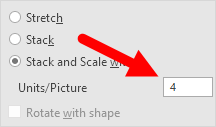
In the same pane, choose Stack and Scale with and enter a value in Units/Picture, for example 10 if each icon should stand for 10 employees. With Stretch or plain Stack, the number of icons doesn’t follow your values, so readers can’t count them.
Use a PNG icon with a transparent background so no white box shows around each picture. In Microsoft 365 you can skip the download: add an icon from Insert → Icons, copy it with Ctrl + C, then click Clipboard in the picture fill options.
To give each bar its own icon, click a bar once to select the series, click it again to select that bar alone, then apply the picture fill.
For a chart that switches between groups, add option buttons from Developer → Insert → Option Button (Form Control), right-click one and set Format Control → Control → Cell link. All option buttons on a sheet share that one cell. Feed the chart from a helper column such as =VLOOKUP(A9,$A$1:$E$6,$A$8+1,0), with the table range locked so it stays put when you fill down.
If you know how to present data in an understandable and effective way, you can deliver your message strongly. For this purpose, one of my favorite things is a PICTOGRAPH. In Excel, creating a pictograph is quite simple and easy.
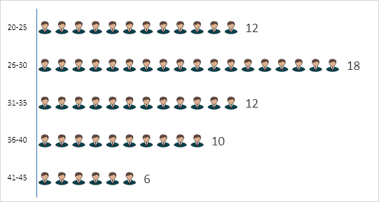
Today in this post, I’d like to share with you a simple step-by-step process to create a pictograph in Excel. Here my idea is to present the number of employees from various age groups in a company.
Now without any further ado, let’s get started.
Simple Steps to Create a Pictograph in Excel
We will use the data below for this chart, and you can download it from here to follow along. As I said, it’s the total number of employees in a company by age group, and we need to present these groups using this chart.
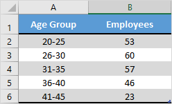
But before we start, we need an icon to use in this chart, and you can download it from a free icon site.
- First of all, just select your data to create a bar chart. For this, go to Insert ➜ Insert Column or Bar Chart ➜ 2-D Bar ➜ Clustered Bar.

- After that, select the data bars in the chart and go to Right Click ➜ Format Data Series.

- From here, go to the “Fill” section and select the “Picture or texture fill” option. Once you do this, you’ll get the Picture source buttons (Insert and Clipboard).

- Now it’s time to insert the picture. Click on the “Insert” button, choose “From a File”, and upload the image you have downloaded.
- Once you insert the image, you have three more options to show that picture in the chart. [Select the third option]
- Stretch – A single image will stretch in the data bar.
- Stack – You will get stacked images in the data bar.
- Stack and Scale with – Images will be shown as per the data (one image for each unit you specify).
Boom! Our chart is ready to rock.
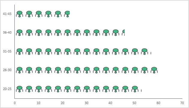
Note: There is an option to specify a unit/picture for the chart. You can use it if the values per bar in your chart are large (more than 20). The thing is that the picture icons become smaller with bigger numbers, and this option helps in that case.
You can also use a different picture for different bars, just like I have used in the chart below.
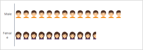
Select each data bar separately and insert a picture one by one for all the bars.
Dynamic Pictograph in Excel
I always love to create interactive charts and this time I want to convert this PICTOGRAPH into a chart in which we can use data dynamically, just like below.
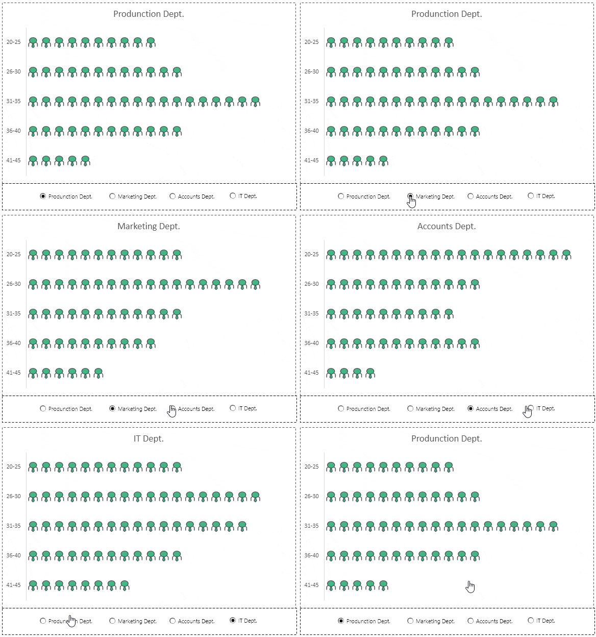
Look at the data below, where we have the same company’s employee data, but department-wise, and we need to create a dynamic chart here which we can operate with option buttons.
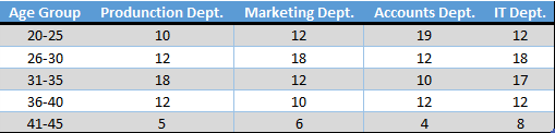
You can download this file from here to follow along, and now use the steps below to create a dynamic pictograph.
- First of all, create a different table with two columns, just like I have below.

- Now, insert four option buttons in your worksheet. For this, go to Developer Tab ➜ Controls ➜ Insert ➜ Option Button (Form Control).
- After that, connect those option buttons with a cell. In my case, I’m connecting them with cell A8.

- Since we need to control the data (department-wise) with option buttons, make sure to name all the buttons according to the department names.
- From here, insert the formula below into the first cell (heading) to the last cell of the second column of the new table.
=VLOOKUP(A9,$A$1:$E$6,$A$8+1,0)

- At this point, we have a dynamic table where we can get data by using option buttons.

- In the end, select this table and insert a bar chart and convert it into a pictograph using the steps you have learned.
Hurray! Our dynamic pictograph is here.
Here’s the lookup formula for the dynamic table so you can copy it. The table range is locked with $ signs, so it stays the same when you copy the formula down, and $A$8+1 picks the column of the department you have selected with the option buttons:
=VLOOKUP(A9,$A$1:$E$6,$A$8+1,0)
Use Excel Icons in a Pictograph
In Microsoft 365, you don’t need to download an icon from a website. Excel has a built-in icon library you can use for the chart:
- First of all, go to Insert ➜ Illustrations ➜ Icons, search for an icon (like “person”), and insert it into the sheet.
- After that, select the icon and copy it with Ctrl + C.
- Next, select the data bars, open Format Data Series ➜ Fill ➜ Picture or texture fill, and click the Clipboard button.
- In the end, select Stack and Scale with and delete the icon from the sheet.
In-Cell Pictograph with REPT
If you just need a quick picture of the numbers without a chart, you can repeat a symbol in a cell with the REPT function. The following formula shows one square for every 5 employees in cell B2:
=REPT("■",B2/5)
REPT ignores the decimal part of the number, so 12/5 shows two squares. Change the 5 to the number of employees one symbol should stand for.
Frequently Asked Questions
Why is my picture stretched in the bar?
Because the Stretch option is selected, which is the default. In Format Data Series ➜ Fill, select Stack or Stack and Scale with to repeat the picture along the bar.
Can I make a pictograph with a column chart?
Yes. The steps are the same: insert a clustered column chart instead of a bar chart, and the pictures stack from the bottom up.
Why do I not see the Developer tab?
It’s hidden by default. Go to File ➜ Options ➜ Customize Ribbon and tick Developer to show it, and then you can insert the option buttons.
Thanks a lot sir. Its a very good representation technique but can it be exported to PowerPoint such that you dont have to use keypads or mouse to click but automatically happens when using pointer?
Puneet , it’s my first time visit to your page , i can see passion in presenting the knowledge to others , I really enjoyed exploring and watching your words
Very well sir and learning a lot from your emails which I am receiving.
Thanks a lot sir.
Great 🙂 Sir I have learnt alot from you. Thanks for your efforts.
Very nice one Puneet. I have a small doubt while creating these option buttons, do I need to create each option button separately?
the ‘Download this sample file from here link’ does not appear to be working. Please help I am really looking forward to experimenting with this chart it looks awesome.
Thank you
I liked very much, congratulations
Sir, Thanks for your post. but i am struggle with option box connect with cell . finally i refer website and make it clear. Please do mention in this post.
OMG!!!! I really love it!!!
Hey Puneet, How can i make graph like the one showing at start of topic at this page “Employee Structure Age Wise”?
Download sample file from above link.
I appreciate your kindness ، it is great and useful.
Really useful and interesting post. I had not thought it before
Thanks Javier Blanco.
This is wonderful! You have the most awesome Excel site, ever!!
Hello Brenda Geoge,
Thanks for your words.