Extract Data for Last N Days (Latest Days) using Power Query (EXCEL)

This tutorial is going to change the way you prepare your data that you use analysis and dashboards.

You are going to learn to use Power Query to extract data for the last N days dynamically.

In this file, you can see that we have this dashboard that I’m controlling with a single cell where you can enter the number of days for which I want the data.

So, when I enter 30, it gives me data for the last 30 days, and when I enter 10, it gives me data for the last 10 days.

This is how this dynamic table and data extraction work. In this tutorial, I’ll show you how to set up this small but powerful way to extract data using Power Query.

Step 1: Create a Query to have a Dynamic Value for the Last N Days

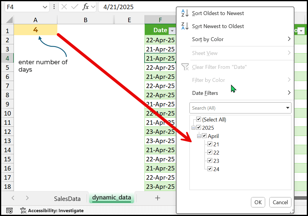
In the first part, you need to have one cell where you are going to add the number of days.

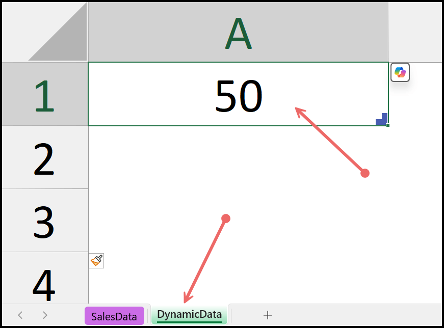
For this, you need to add a new worksheet and name it “DynamicData”, and then in cell A1, where you have the value that you need to use to enter the number of days.

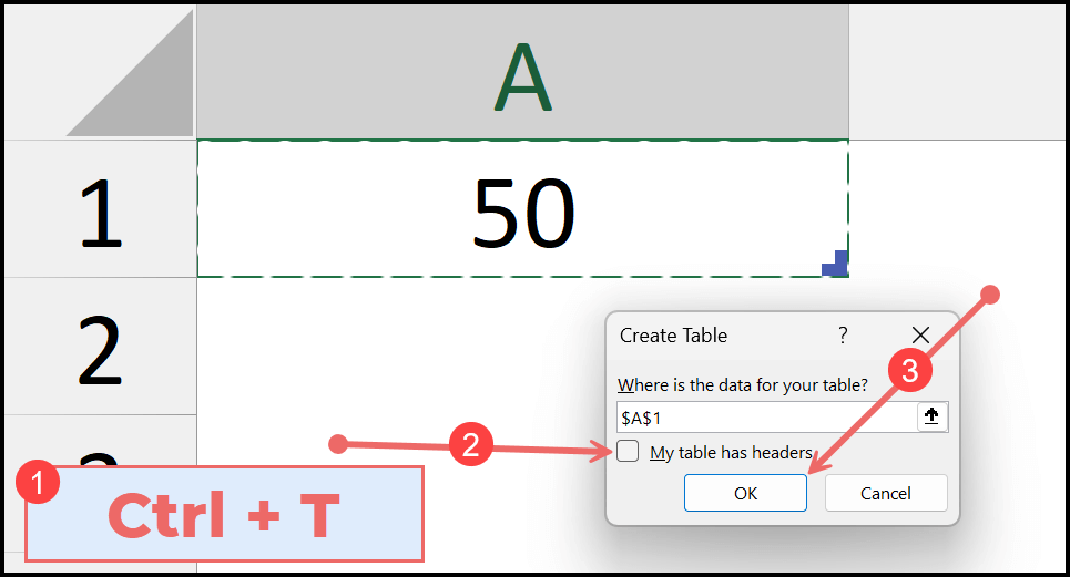
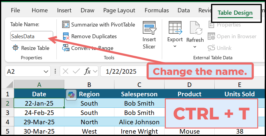
Now you need to convert this single cell into an Excel table that you can load into the Power Query editor.

For this, use the keyboard shortcut Control + T, and then in the Create Excel Table dialog box, make sure that “My table has headers” is unticked, and after that, you need to click on OK to apply the table.

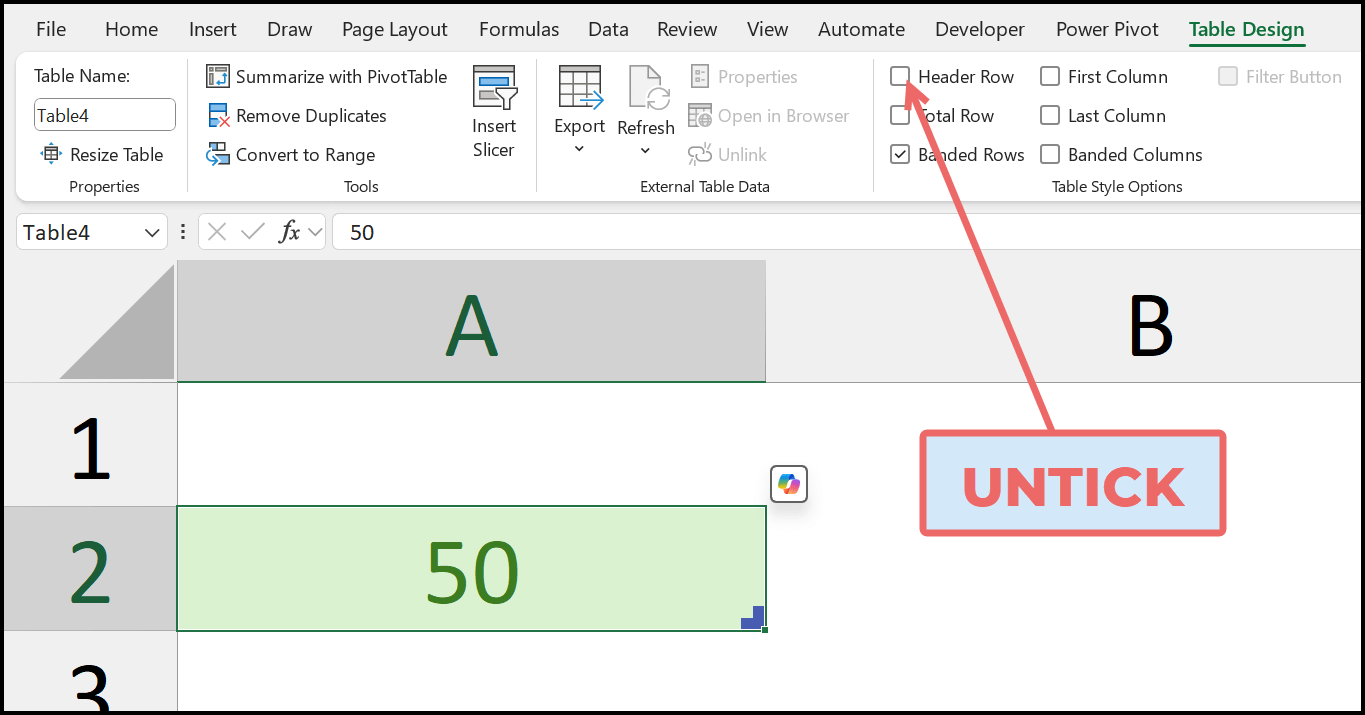
From here, click on this design tab, and then untick the header row checkbox.

This will remove the header from the table that you have with a single cell. Here you can see the value that was in cell A1, now it is in cell A2.

Move this small table from A2 to A1 (simply drag this cell from A2 to A1).

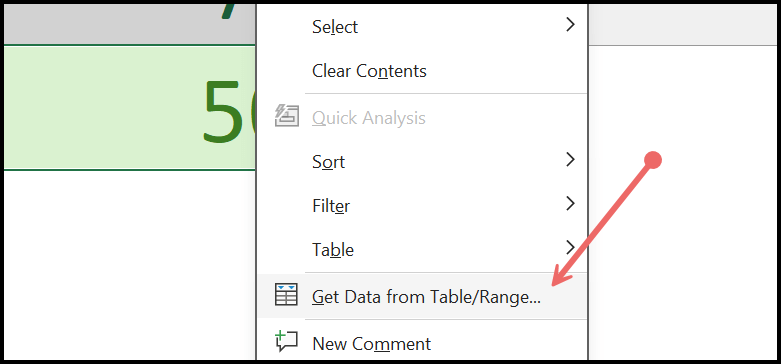
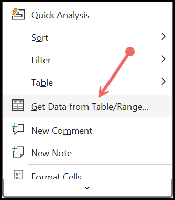
And now you need to right-click on the cell, and then click on the option that says, “Get data from Table/Range”. The moment you click on this option, it will load your single cell into the Power Query editor.

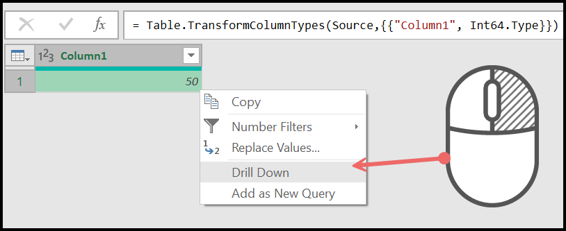
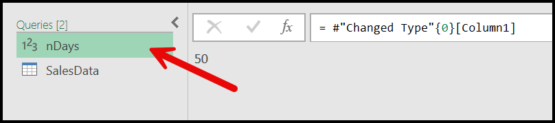
In the Power Query editor, you need to convert this single-cell table into a number.  Right-click on the cell and use the option “Drill Down”. It will convert your table into a single number, that is 7.

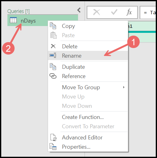
Now, right click on the query name from the left side and select the option “Rename” and then rename it with the new name “nDays” or any name you want.

At this point, you have this query that has value from a single cell from a worksheet, and we’re going to use this query as a dynamic value to extract data for the last N days.

If you enter 10 in the cell you have in the worksheet, you’ll get data for the last ten days.

If you enter 7, you’ll get data for the last seven days. This cell becomes your dynamic controller that helps you extract data based on the number of days you specify.

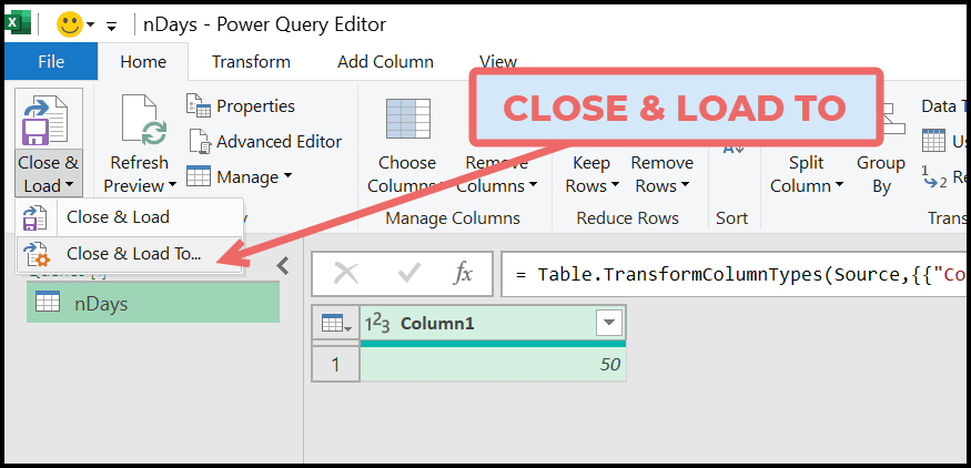
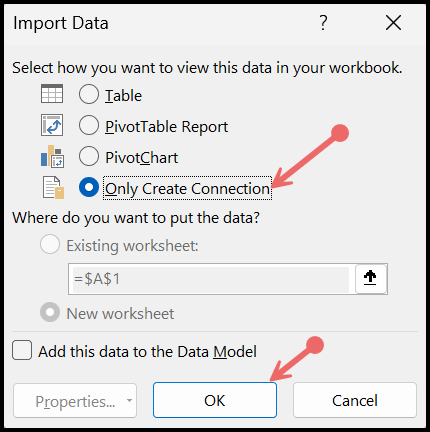
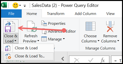
Right now, you’re in the Power Query editor, so you need to load this data as a connection. To do that, go to the Home tab, click on the “Close and Load” drop-down, and then select the “Close and Load to” option.

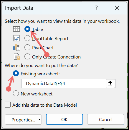
Now, from the “Import Data” dialog box, you need to click on the “Only Create Connection” option, and after that, click OK.

You can see on the right side of your Excel window that you have this connection for the query that you have just created in your Power Query editor.

Read Also: Concatenate Values in Power Query / Remove Duplicates using Power Query

Step 2: Load Main Data into the Power Query Editor

Next, you need to go to your main data that you have in the worksheet SalesData and then convert that data into an Excel table (Control + T) and name that table “SalesData”.

And now the right-click by selecting any cell from the table and click on “Get Data from table/Range”. Once you do that, it will instantly load your main data table into the Power Query editor.

Before you move ahead, you can see in your table that you have in the Power Query editor, right now, the date column has time as well.

But we only need the date instead of the date and time, so we need to correct this, and for this, you need to select the date column and then go to “Transform, Tab”.

From the transform tab, click on the “Date” dropdown, and after that, select the “Date Only” option.

This will convert the date column from date and time to only dates.

Step 3: Add a Custom Column with a Conditional Formula to Test Dates

Now you need to add a custom column with a conditional formula that can test if the dates that you have in the date column are within the range of the days for which you want the data.

Let’s say if I want data for the last seven days, we need to create a condition that can test if the dates are within that range.

This conditional formula will return TRUE for the dates that are within the range of the last seven days and FALSE for all the dates.

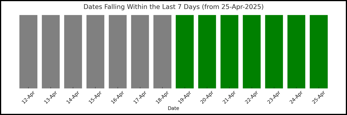
So, if today is the 25th of April 2025 and if I specify 7 for the last 7 days, that means the range of dates is 24-April to 18-April 2025, and this formula will return true for all these dates we have in this range and FALSE for all the other dates.

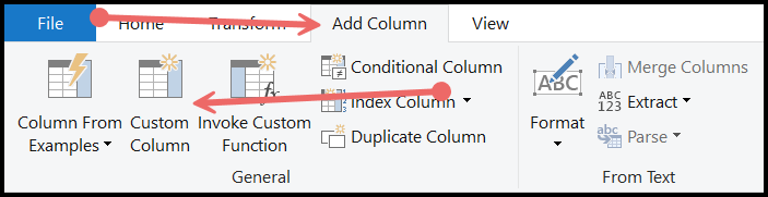
To insert a new custom column, go to the “Add Column” tab and click on the Custom Column button. This will open a new dialog box where you can insert a formula to add a custom column.

Now, in your custom column dialog box, first, you need to enter a new name, and for this, you need to enter the name “lastNDAYS” or any name that you want to give to your custom column.

And after that, in the custom column formula input box, you need to enter the following formula that allows you to create a condition that tests a condition from the dates that you have in the date column.

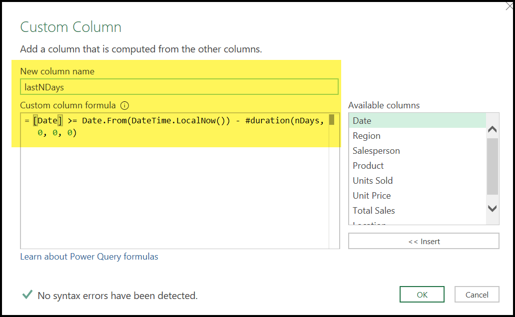
=[Date] >= Date.From(DateTime.LocalNow()) - #duration(7, 0, 0, 0)

And in the end, click OK to add the custom column.

Step 4: Make the Custom Column Formula a Dynamic Formula

At this point, you have a custom column in your data that returns TRUE for the dates that are within the range of the last seven days and FALSE for the rest of the dates.

Now you need to make this formula and this custom column dynamic, so that you can change the number of days, I mean the range of the dates, whenever you want.

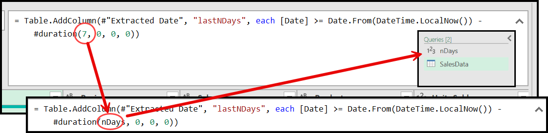
If you remember, at the start we created a query from a single cell from the DynamicData worksheet, and now we are going to use that query as a dynamic input for the days in this formula.

What will happen now, when you change the number of days from the worksheet, this custom conditional formula will use that number to create a range of dates, and this way your formula will work dynamically based on the value you enter in the cell.

First, click on the small downward arrow that is on the right side of your formula bar. There, you can see that you have this formula that you have added to your custom column.

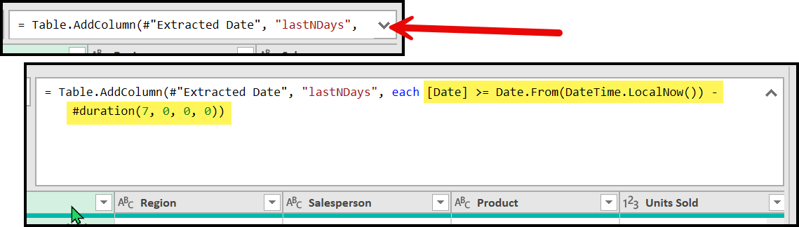
And in that formula, you have a number which is 7. Now, instead of this number, we need to use the query to make this value dynamic.

So, you need to replace that number with the name of the query “nDays” which is the query we have created from the worksheet cell. In the end, HIT “Enter” to apply the formula.

Step 5: Filter TRUE Values and Remove the Custom Column

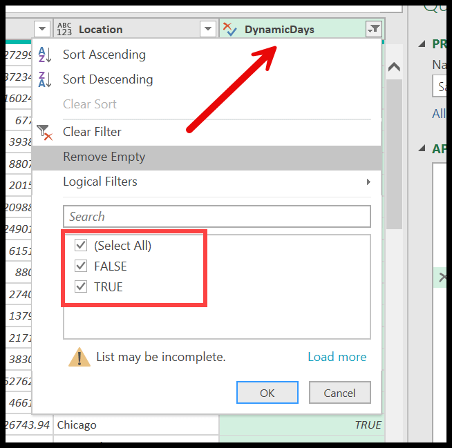
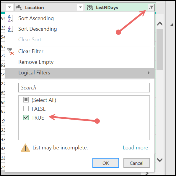
At the end of the table, you have a conditional column that shows true or false based on the value you entered in the worksheet cell.

But you only need the rows where the value is TRUE, meaning those entries that fall within your selected date range (last N days).

So, click on the filter icon, untick FALSE, and then click OK.

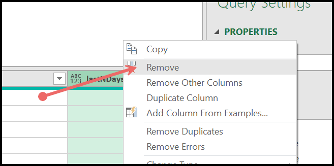
Now that your column is filtered, you only have values where you have true in the custom column. But now we are going to do something, and that is to delete this custom column.

I’m sure you are going to be surprised, why I’m telling you to delete this column, but trust me, you are on the right path.

Right-click on the column header and click the option to remove the column.

Let me tell you this again, when you remove the column, it will not affect the filtration that you have done in the last step, your data is still filtered with the rows where you have the value TRUE.

Step 6: Load Data Back to the Workbook

Your data is ready, and now you need to load this data back into your workbook. Go to the home tab and click on the “Close and load” dropdown, and then click on “Close and load to”.

From the Import Data dialog box, click on the “Table” option, and then click on the “Existing Worksheet”, and then specify any cell from the worksheet “DynamicData”. And in the end, click OK to load the data.

Step 7: Test IF Your Data is Dynamic or Not

At this point, everything is ready, and you need to test the data. For this, you need to change the value in cell A1, and then you need to click on the refresh all to refresh everything, and then you need to check if the data in the table has changed or not.

If you have the value 7 in the cell, that means data for the last seven days, and you change it to 4, and when you click on the refresh all button, you need to check if you are getting data for the last 4 days.

Or if you change the number from 7 to 10 and then you need to check if you are getting data for the last 10 days. This is something you need to verify to make sure that your data is getting extracted using the value that we have in cell A1.

Step 8: Insert a New PIVOT TABLE

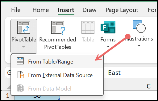
Now, at this point, your dynamic data is ready, and the next thing is to insert a pivot table using this data. First, select any of the cells from the data and then go to your Insert tab, and after that go to Pivot Table dropdown and then click on the option from table or range.

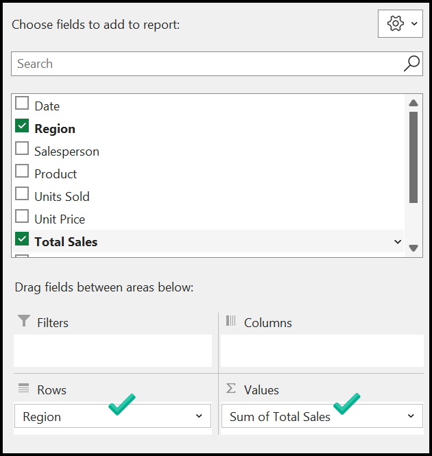
To create this pivot table, add the Region column to the Rows field and Total Sales to the Values. Or you can create a pivot table the way you want.

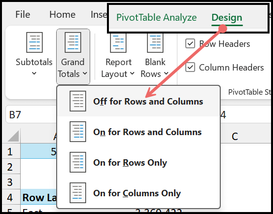
There is one small tweak that we need to do on your pivot table, and that’s removing the grand totals. Go to the design tab and from the layout group, click on the Grand Total dropdown. And from this dropdown, turn off the grand totals.

Your Pivot Table is ready.

Related Read: VBA to Create a PIVOT TABLE Single + Multiple Pivots

Step 9: Small Adjustment to Make Refresh Pivot and Data Table Together

Before you start using a Pivot Table with a dynamic data table, you need to make a little adjustment.

When you click on the refresh button, it refreshes both the data table and the pivot table at the same time, but here’s the problem: the data table needs to be updated first, and only then can the pivot table be refreshed, since both happen together.

Since the table doesn’t wait for the data table to finish updating, it ends up using the old data.

To fix this, you need to make sure the data table is refreshed first, and only after that, the pivot table refreshes so that it picks up the latest data correctly.

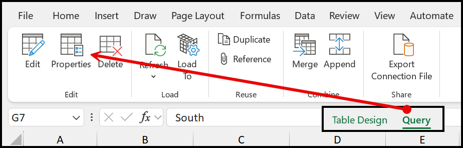
This tweak is quite simple; you need to go to the Query tab and then click on the “Properties”.

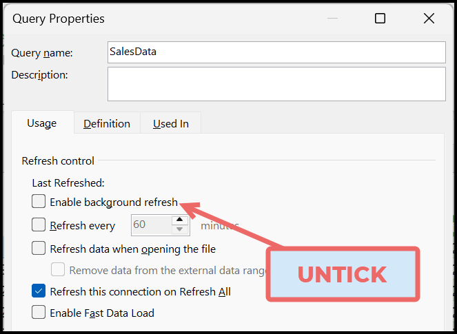
From the properties dialog box, untick the option “Enable Background Refresh”.

Step 10: Insert Pivot Chart from the Pivot Table

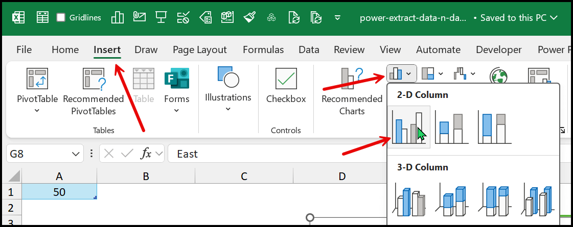
The final step is to insert a column chart from the pivot table. If you already know how to create a Pivot Chart, you can skip this step and insert the chart directly when you create the pivot table.

To insert a chart, select any cell from the pivot table, go to the Insert tab, open the Insert Column or Bar Chart drop-down menu, and choose a 2D column chart.

After inserting the chart, you can apply your formatting or use the formatting from my sample file.

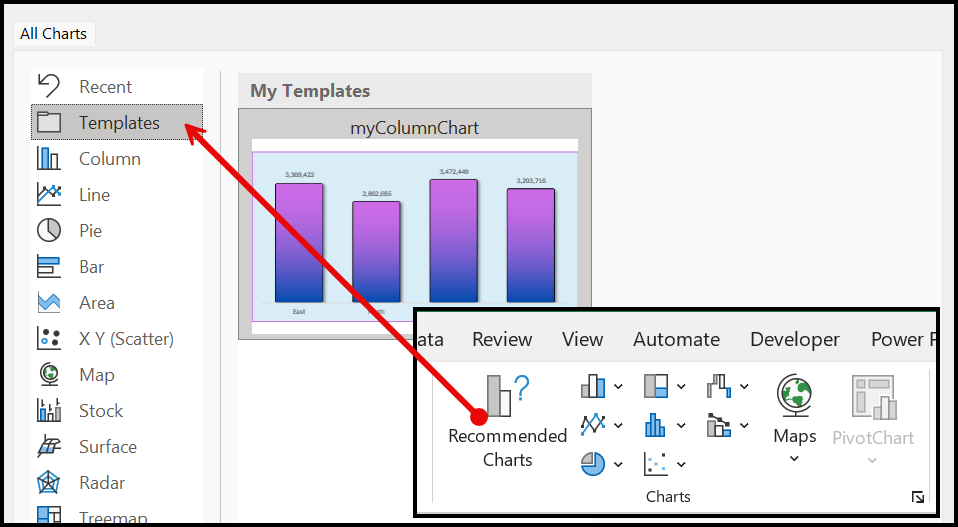
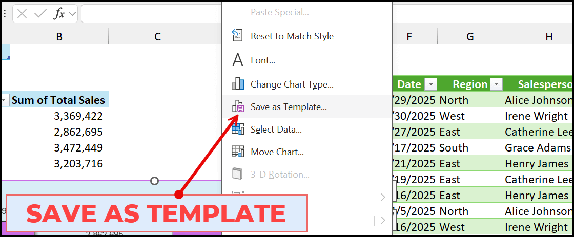
The easiest way to use the formatting I have used is to save my chart formatting as a template. To do that, open the sample file, select the column chart, right-click on it, and select “Save as template…”.

This way, you will save the formatting as a template, and then you can apply that template when creating a new chart in your file.

Go to the Insert tab, click recommended charts button and then from the Templates, insert the chart with the formatting.