What is Not Equal Operator in Google Sheets?
Like Microsoft Excel, in Google Sheets, the “Not Equal” operator is used to compare two values and determine if they are different. The syntax for the “Not Equal” operator is <>. It indeed combines two operators: “greater than” (>) and “less than” (<). To enter it, you can use the key on the keyboard.

A1 <> B1 This checks if the value in cell A1 is not equal to that in cell B1. If the values are different, the result is TRUE. If the values are the same, the result is FALSE.
Use Not Equal with the IF (Conditional Formula)
The not equal is often used in IF to test conditions. Let’s say you have a list of students and their grades, and you want to mark those who did not get an “A” as needing improvement.
=IF(B2 <> "A", "Needs Improvement", "Excellent")
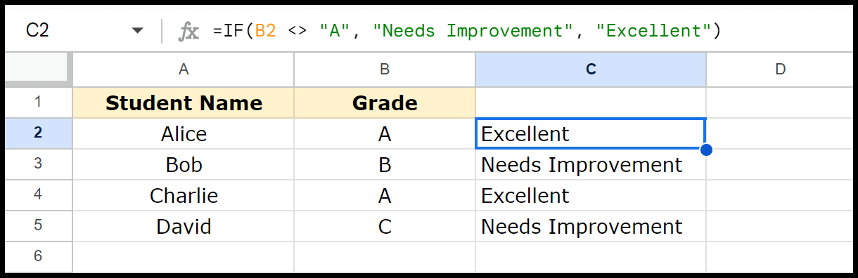
Here, IF checks whether a condition is true or false and returns one value if true and another value if false.
- B2 <> “A” – This condition uses the not equal operator (<>) to check if the value in cell B2 is not equal to “A”. If the grade in B2 is anything other than “A”, this condition is true.
- IF(B2 <> “A”, “Needs Improvement”, “Excellent”) – If condition B2 <> “A” is true (meaning the grade is not “A”), the formula returns “Needs Improvement”, and if the condition is false (meaning the grade is “A”), the formula returns “Excellent”.
The formula categorizes students based on their grades, marking those with grades other than “A” as needing improvement and those with an “A” as excellent.
Read Also – Greater Than or Equal To in Google Sheets
Using Filter Function with Not Equal
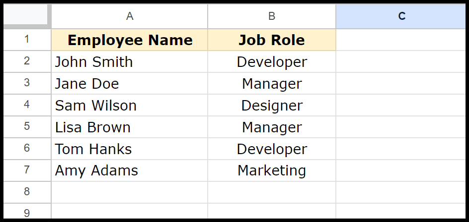
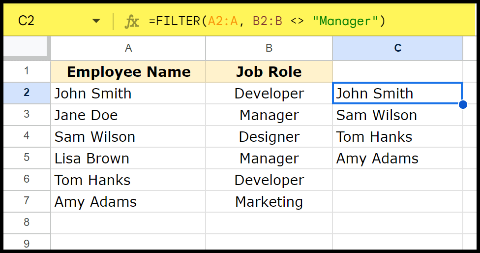
Let’s say you have a list of employees and their job roles in a Google Sheet. You want to find all employees who are not managers so you can invite them to a training session. To do this, you can use the “Not Equal” operator, represented by <>.
In our example, we have employee names in column A, and their job roles in column B; you can use a formula like =FILTER(A2:A, B2:B <> “Manager”). This formula will create a list of all employees whose job roles are not “Manager”.
Combine SUMIF with Not Equal Operator
When you use SUMIF with the not equal operator, you can sum values based on criteria where the values do not match a specified condition.
Let’s say you have a sales report listing products and their sales amounts. You want to sum the sales amounts for all products except those labeled “Widgets”. To sum the sales for all products except “Widgets”, you can use the below formula:
=SUMIF(A2:A6, "<>Widget", B2:B6)
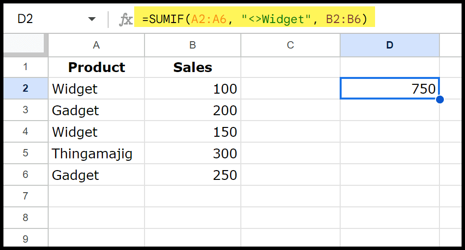
When using the Not Equal (<>) in the SUMIF, enclosing text values in quotation marks is important. In the above formula, we have used “<>Widget”, but you can also write it as “<>” &” Widget”.
Using Not Equal with Conditional Formatting
Let’s say you want to apply conditional formatting to a cell to highlight if any value is entered rather than a specific value. So, for this, select the cell you want to format, apply the formatting, and then go to Format > Conditional formatting.
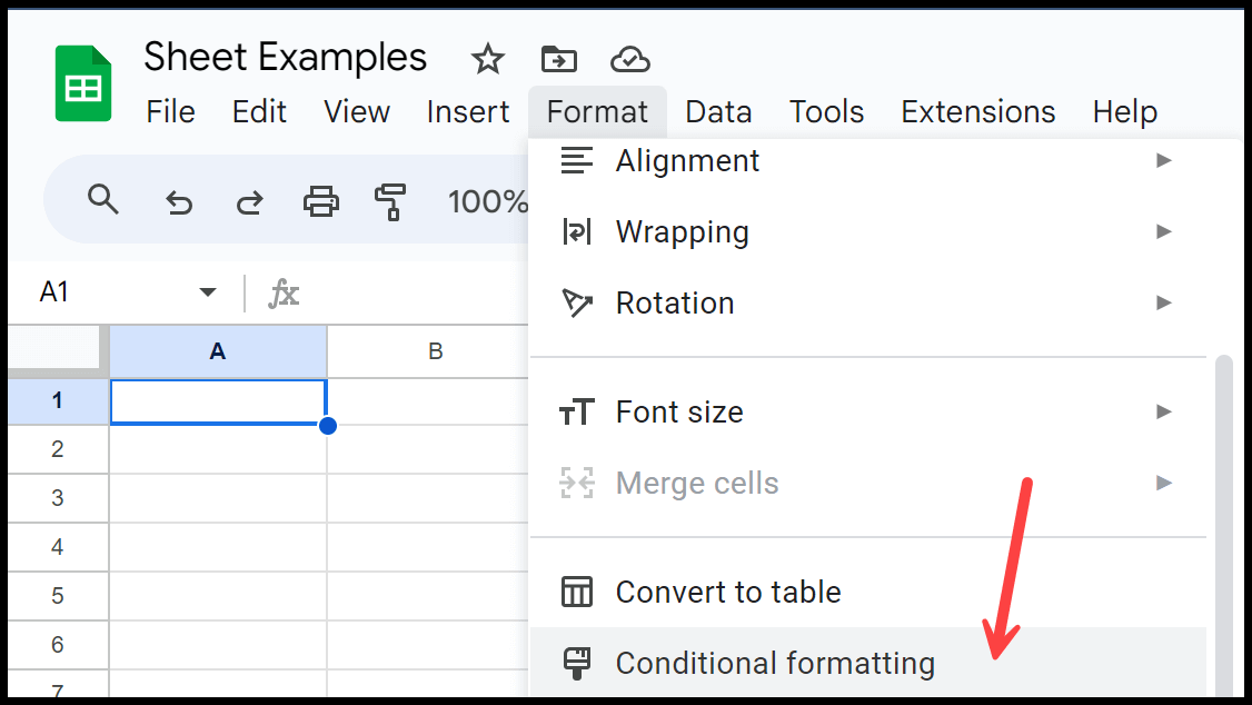
Now, click on the “Add Rule”, and then select “Custom formula is” from the “Format cells of” drop down. And then, in the input bar, enter the formula =A2<>”Yes”, and specify the color for the cell applied when the condition is met. In the end, click Done to apply.
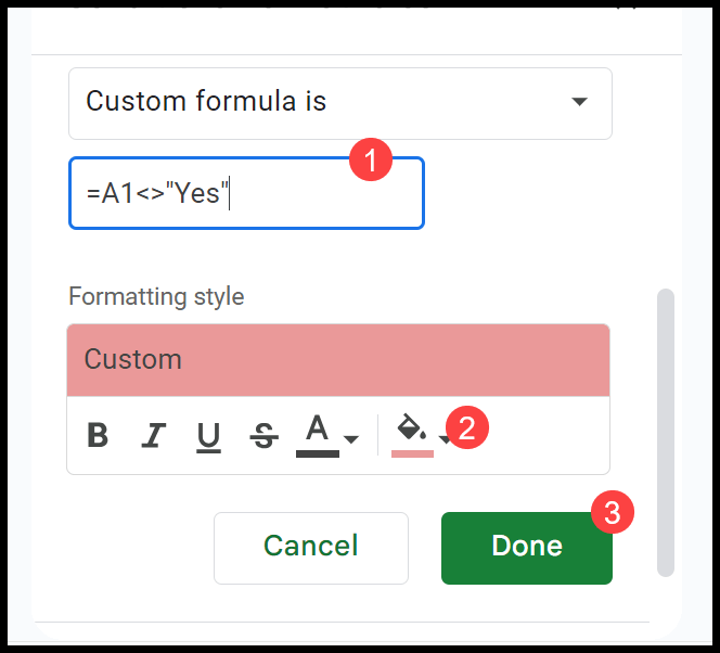
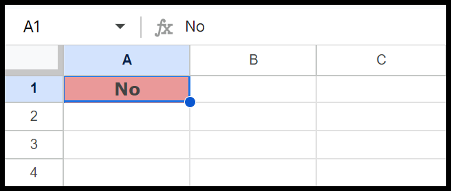
Now, when you enter a value in cell A1 other than “Yes,” the red cell will be applied to it.
Read Also – Highlight Duplicates in Google Sheets
Using Not Equal with IFERROR
To handle cells where the sales data might be missing or result in an error (like division by zero) and provide a custom message if an error occurs, you can use IFERROR with not equal.

=IFERROR(IF(C2 <> 0, (C2 - B2) / B2, "No Sales Data"), "Error in Calculation")
First, it checks if the current period’s sales (in cell C2) are not equal to zero (C2 <> 0). If the sales are not zero, it calculates the sales growth by subtracting the previous period’s sales (in B2) from the current period’s sales, then dividing by the previous period’s sales to get the growth percentage (C2 – B2) / B2).
IFERROR ensures that if any part of this calculation causes an error (like if B2 is zero, causing a division by zero error), it will return “Error in Calculation” instead of showing an error.
Check Non-Blank Cells with Not Equal
You can use COUNTA to count non-blank cells; you can write specific formulas using COUNTIF and <>. See the below example:
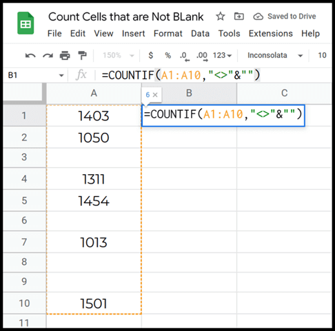
=COUNTIF(A1:A10,"<>"&"")
COUNTIF counts the number of cells in a range that meets a specific condition. In this case, the range is A1:A10. The condition is “<>” & “”, which might look a bit strange, but it simply means “not equal to an empty string”. So, the formula is counting all the cells in the range A1 to A10 with something in them, anything that’s not blank.
Combining with ARRAYFORMULA
You can use the not equal within an ARRAYFORMULA to apply conditions simultaneously across a range of cells. Let’s say you want to check if multiple columns meet a not-equal condition. If you have two columns (A and B) and you want to find rows where values in column A are not equal to values in column B:
=ARRAYFORMULA(A2:A10 <> B2:B10)
This formula returns an array of TRUE or FALSE, showing which rows have different values in columns A and B.
Using Not Equal with AND & OR Functions
The not equal (<>) with AND and OR can help you create more complex logical conditions. Here are some examples that you can check out and learn. To find employees not in the “Sales” department and not “Managers”.
=AND(A2 <> "Sales", B2 <> "Manager")
=IF(AND(B2 <> "Sales", C2 <> "Manager"), "Yes", "No")
To find employees not in the “Sales” department or not “Managers”.
=OR(A2 <> "Sales", B2 <> "Manager")
=IF(OR(B2 <> "Sales", C2 <> "Manager"), "Yes", "No")