While working with functions and formulas in Google Sheets, it is obvious that you get an error in the result instead of the value at some point. Let’s say you use VLOOKUP in a worksheet, which returns an #N/A! error as the value you are looking for is not in the data. In this case, you can use the IFERROR function to convert that error into a meaningful value.
What is the IFERROR Function?
The IFERROR function is a logical function that is useful for handling formula errors. You can wrap your formula into IFERROR and specify a value to return if an error occurs. Or, if no error is returned in the result, you get the result as it is.
Syntax
Here’s the syntax of the IFERROR:
=IFERROR(value, [value_if_error])
- value: This is the formula or expression you want to check for errors.
- value_if_error: You want to show this if you have defined an error formula in the first argument. It is also an optional argument. So, if you skip specifying this argument, Google Sheets will show a blank cell when an error occurs.
Example to understand IFERROR in Google Sheets
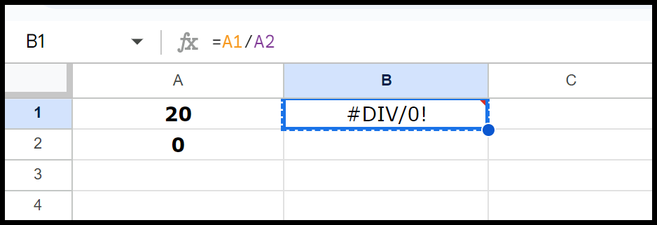
In the below example, we need to divide 20 by a zero. As you know, when you divide any number by 0, you get a #DIV/0! Error.
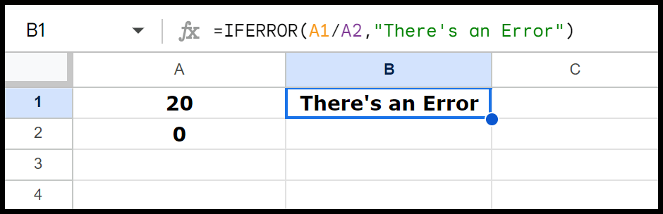
But when you wrap the formula into the IFERROR function and then specify a value to get if the error occurs, it returns that value in the result instead of the error. With IFERROR, you get “There’s an Error” in cell B1, making it clear something went wrong in a more understandable way.
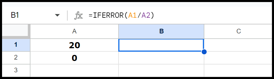
As I mentioned earlier, if you skip specifying the value_if_error then it shows you a blank value in the cell if an error occurs in the result.
Errors that IFERROR Can Handle
The IFERROR function can handle several types of errors. And the best way is to use it with all the formula where you have a high chance of of getting an error in the result.
- #DIV/0!: Division by zero error, occurs when a number is divided by zero.
- #N/A: Value Not Available error, typically seen in lookup functions when a value isn’t found in the data.
- #REF!: Reference error occurs when a cell reference is invalid, like deleting cells, rows, and columns used in a formula.
- #VALUE!: Value error happens when the wrong type of argument is used in a function.
- #NUM!: Number error, occurs when a formula has invalid numeric values, like taking the square root of a negative number.
- #NAME?: Name error happens when Google Sheets doesn’t recognize a formula or range name.
- #NULL!: A null error typically occurs when an attempt is made to intersect two areas that do not intersect.
Limitation that comes with IFERROR
IFERROR is an amazing formula, but it has a few limitations that you need to consider while using it.
- Can’t Differentiate Errors: IFERROR handles all errors without distinguishing between them. This means you can’t customize messages for different kinds of errors.
- Single Alternate for all the Erros: IFERROR allows only one alternative value or message to display, regardless of the error type.
- No Error Information: It doesn’t explain why the error occurred, making it harder to debug sometimes.
- Performance in Large Data: In large data, IFERROR can slow down performance by calculating each formula twice—once for the actual result and once to check for an error.
Even though there are some limitations to IFERROR, it’s helpful to use it with formulas.
More Examples to understand IFERROR
Here are a few examples to help you understand how to use IFERROR with other functions.
1. IFERROR for Checking the Number
Now, let’s say you want to convert a text (which is a number) into a number; you can use IFERROR there to check if that can’t be converted.
=IFERROR(VALUE(A1), "Invalid number")
2. IFERROR with IF
And in the same way, you can use nested IFERROR for multiple conditions. You can nest IFERROR within other functions or even another IFERROR to handle more complex conditions.
=IFERROR(IF(A1 >= 100, A1/B1, "Value too low"), "Error or too low")
If A1 is not greater than or equal to 100, it will show “Value too low”. If there is any error in dividing A1 by B1, it will show “Error or too low”.
3. IFERRROR for Custom Calculations
And here’s how you can use IFERROR with custom calculations.
=IFERROR(A1/B1, A1 + B1)
If there is an error in dividing A1 by B1, it will instead show the sum of A1 and B1.
4. IFERROR with ARRAYFORMULA
Now, if you combine ARRAYFORMULA with IFERROR, you have a powerful way to handle errors efficiently across a range of cells.
=ARRAYFORMULA(IFERROR(A1:A10 / B1:B10, "Error"))
The above formula applies the division operation across the range from A1 to A10 and B1 to B10. If an error occurs in any cell (like dividing by zero), it displays “Error” instead.
Let’s say you want to subtract the values in column B from the values in column A, and if there’s any error (e.g., non-numeric values), you want to display a custom message.
=ARRAYFORMULA(IF(ISERROR(A1:A10 - B1:B10), IF(ISNUMBER(A1:A10) = FALSE, "Invalid number in A", IF(ISNUMBER(B1:B10) = FALSE, "Invalid number in B", "Calculation error")), A1:A10 - B1:B10))
The formula checks for errors when subtracting values in column B from values in column A. If there’s a problem, such as non-numeric values in the cells, it helps you determine what’s wrong. ISERROR(A1:A10 – B1:B10) looks for any errors in the subtraction.
If it finds an error, IF(ISNUMBER(A1:A10) = FALSE, “Invalid number in A”, IF(ISNUMBER(B1:B10) = FALSE, “Invalid number in B”, “Calculation error”)) check why so.
5. IFERROR to Check Cell Value
Use IFERROR when you check if a cell contains a value you specify.
=IFERROR(SEARCH("text", A1), "Not found")
In this formula, SEARCH looks for the word “text” within the value of cell A1. If it finds the string, it returns the position of the first letter of “text” within the cell. Now, here’s where the IFERROR part comes in.
If the SEARCH function can’t find the word “text” in A1, it usually gives an error message. To avoid that, IFERROR steps in and catches the error. Instead of the error message, it shows the phrase “Not found”.
Alternative to IFERROR
IFERROR is the best way to handle errors in Google Sheets, but there are a few alternatives that you can consider while working with formulas.
- IF and ISERROR: You can use the IF in combination with the ISERROR to check for errors and show a value or message. Example:
=IF(ISERROR(A1/B1), "Error", A1/B1)This formula checks if the division of A1 by B1 results in an error. If it does, it displays “Error;” otherwise, it shows the division result. - IF and ISNA: If you want to handle the #N/A error, use the IF with the ISNA. Example:
=IF(ISNA(VLOOKUP("SearchTerm", A1:B10, 2, FALSE)), “Not Found”, VLOOKUP(“SearchTerm”, A1:B10, 2, FALSE)) It checks if the VLOOKUP function returns an #N/A error. If it does, it displays “Not Found”; otherwise, it shows the lookup result.