Use XLOOKUP with Multiple Criteria in Excel (Formula)

Using XLOOKUP with Multiple Criteria is one of the most powerful and amazing formulas you can write in Excel. In this tutorial, we are going to learn it in detail.

What is the XLOOKUP Function in Excel

The XLOOKUP function is a powerful tool for finding specific data within a range. Unlike older functions like VLOOKUP or HLOOKUP, XLOOKUP is more flexible and easier to use. It allows you to search for a value in one column and return a corresponding value from another, no matter where the columns are located. That means you don’t have to worry about the search column always being on the left side, as with VLOOKUP.

In XLOOKUP, you need to specify three main pieces of information: what you’re looking for (the lookup value), where you’re looking for it (the lookup array), and where you want to find the answer (the return array).

Syntax of XLOOKUP

You can quickly look at its syntax if you have never used the XLOOKUP.

XLOOKUP(lookup_value, lookup_array, return_array, [if_not_found], [match_mode], [search_mode])

• lookup_value: This is the value you want to find. It could be a number, text, or cell reference.
• lookup_array: This is the range of cells where you want to search for the lookup value.
• return_array: This is the range of cells from where you want to get the result.

The above arguments are required, and the three arguments below are optional, so you can skip specifying them.

• if_not_found: This is what you want to return if the lookup value isn’t found. If you leave it out, you’ll get an error if the value isn’t found.
• match_mode: This tells the function how to match the lookup value. You can choose an exact match, an approximate match, or a wildcard match.
• search_mode: This tells the function how to search the lookup array. You can search from top to bottom, bottom to top, or use binary searches for faster results in sorted data.

Using XLOOKUP with Multiple Criteria for Lookup Value

Like any lookup function, you can’t use multiple criteria by default. However, you can create a workaround when using the XLOOKUP function. There are two ways to do that in XLOOKUP. In the below example, we have a list of students with roll numbers, names, and scores.

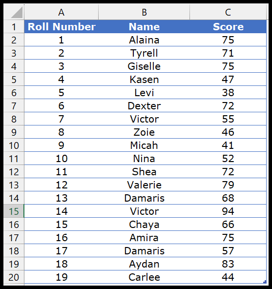
In this data, we need to write a formula that uses two criteria as a lookup value. This is because there’s a chance of having the same student name. But you can see the roll number is a unique value. When you combine the roll number with the name, it creates a unique value to look for.

There are two ways to do this: one is to use the helper column, which is easy to use, and the second is to use two conditions with arrays to create a single array for the lookup array (which is my favorite). In this tutorial, we are going to learn both methods in detail.

1. Multiple Criteria with XLOOKUP (Array Method)

You can use an array if you don’t want to use the helper column. First, let’s write this formula and then learn how it works.

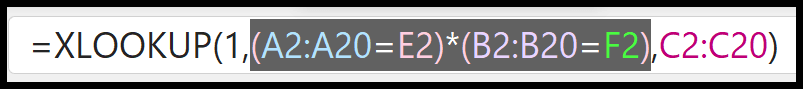
1. Enter the XLOOKUP in a cell, and in the lookup_value, enter 1.
   
2. Now, we need to create an array to look up the roll number in the roll number column and the name in the name column. So, enter (A2:A20=E2)*(B2:B20=F2) in the lookup array.
   
3. After that, in the return_array, refer to the score column.
   
4. In the end, close the function and hit enter to get the result.
   

Arrays are what makes this formula powerful.

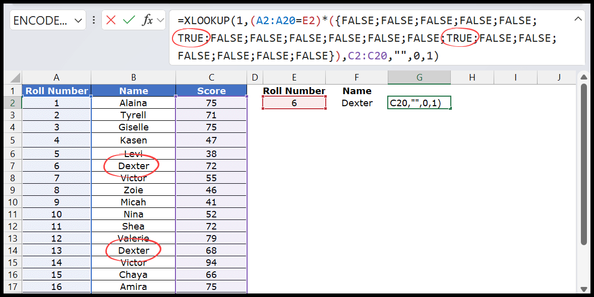
Let’s understand this in detail. In the first part of the array, we tested the roll numbers in the roll number column, and it returned an array with TRUE and FALSE. In this array, we have FALSE, where the roll number does not match the value in cell E2.

We have one value in the cell E2, and we would have one TRUE in the array.

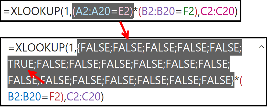
We have TRUE in the sixth position in the array, which is the position of the roll number 6 we are looking up in the roll number column.

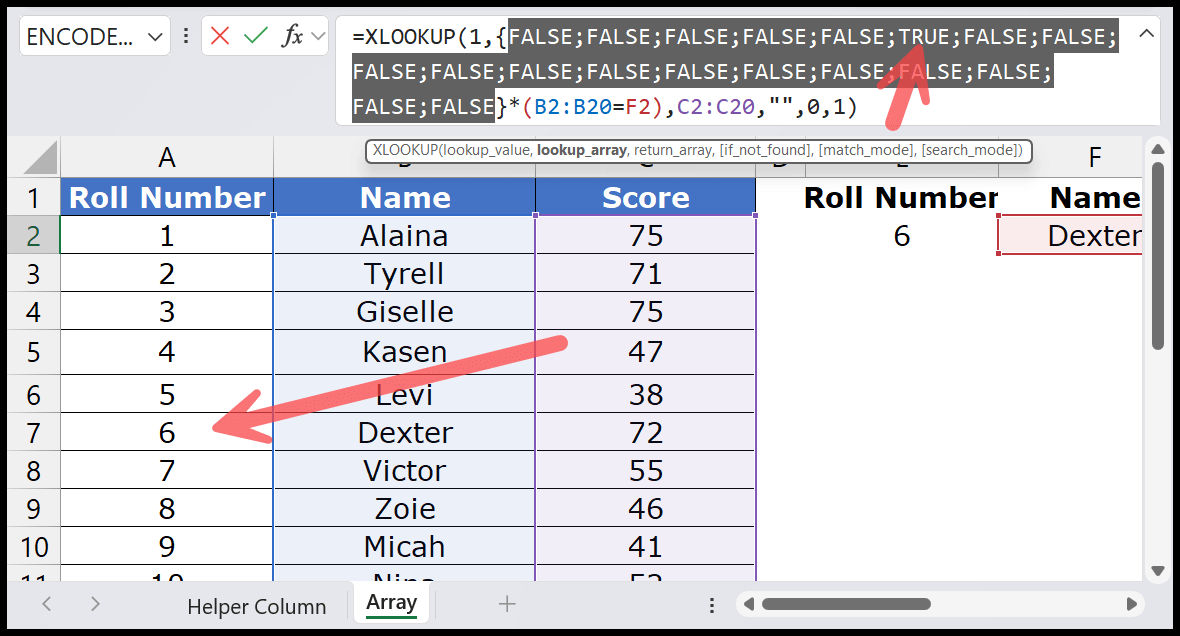
The same is true for the second array, where we have TRUE for the student’s name, “Dexter.” If you look at the data table, the name “Dexter” appears twice.

That means there are two students with the same name. But what makes them unique is their roll number. That’s why we are using multiple criteria so that we don’t get the score of the wrong student even if the student’s name is correct.

Moving forward in the formula, you get a new array with 0 and 1 when you multiply both arrays. In this array, 1 is in the sixth position. And at the 6th position, where you have the roll number 6 and the name “Dexter”

In the lookup value, we have 1 to look up for. Then, the formula goes to the lookup arrays where we have 0 and 1, takes one from there, and returns the score from the range C2:C20.

In the lookup array, 1 is in the sixth position, which means the right student, with roll number 6 and the name “Dexter,” is in row 6 and whose score we have in the result.

As we have further had a few arguments in the XLOOKUP function, you need to specify a blank value if the value is not found in the list, use exact match, and search mode from top to bottom.

2. Multiple Criteria with XLOOKUP (Helper Column Method)

This is a simple way to create a new helper column, combining values from two columns and then creating a lookup value to get the score.

1. First, add a new column to use as the helper column.
   
2. Now, in the helper column, you need to combine the roll number and name of the student.
   
3. After that, create the concatenated value to lookup. Then, in two cells, enter the roll number and name of the student.
   
4. Next, enter the XLOOKUP and combine values from the call F2 and G2 to use as the lookup value in the function.
   
5. From here, refer to the helper column as lookup_array and the score column as a return_array.
   
6. In the end, hit enter to get the result.