THIS FORMULA IS A PURE MAGIC.
If you want to write a SUBTOTAL formula in Excel with IF (condition), you need to use multiple functions to do this. But before we do this, let’s understand the data we have for this example.

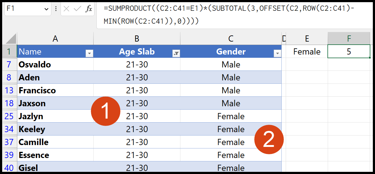
In the above example, you have three columns:
- Name
- Age Slab
- Gender
And when you filter a slab from the Age Slab column, it shows the count of females in cell F1. So that means we have a formula that shows the count of filtered values but with a condition. The formula we have:
=SUMPRODUCT((C2:C41=E1)*(SUBTOTAL(3,OFFSET(C2,ROW(C2:C41)-MIN(ROW(C2:C41)),0))))Understanding SUBTOTAL IF Formula
This formula uses five functions: SUMPRODUCT, SUBTOTAL, OFFSET, ROW, and MAX. Therefore, to understand this formula, we need to split it into multiple parts.
1. ROW(C2:C41)-2,0)
This part of the formula uses MIN and ROW functions.
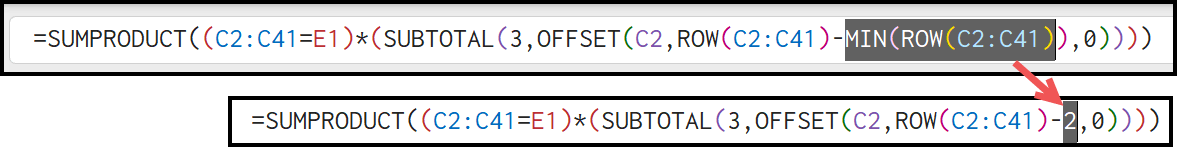
- In the ROW, we have referred to the “Gender” columns, and it returns an array of row numbers.
- After that, MIN takes that array or row numbers and returns the minimum row number. So that’s why we have got 2 in this part of the formula.
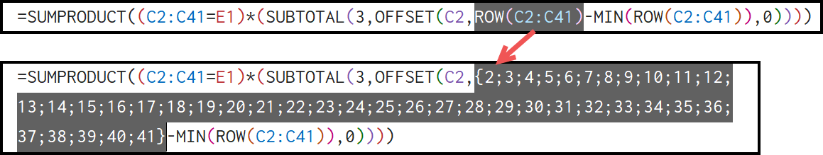
2. ROW(C2:C41)
In this part, we only have the ROW function, which returns an array of row numbers.
3. OFFSET(C2,ROW(C2:C41)-MIN(ROW(C2:C41)),0)
Now we have the OFFSET function. It helps you to create a reference to a range using a cell reference as a starting point. In the reference argument, we have referred to cell C2, the first cell from where our gender range starts.
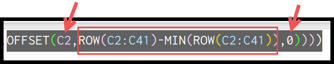
In the rows argument, we have that part of the formula discussed above in the first two parts. After that, in the cols argument, we used 0. With all these, OFFSET returns an array of all the values from the “Gender” column.
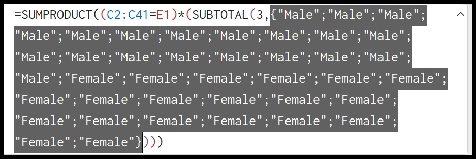
4. SUBTOTAL(3,OFFSET(C2,ROW(C2:C41)-MIN(ROW(C2:C41)),0))
We have used the array returned by the OFFSET in the SUBTOTAL. And in the function_num, we have used 3, which tells SUBTOTAL to use the COUNTA function for calculation.
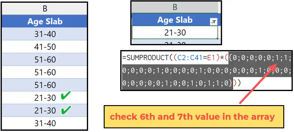
When you use a filter on the column “Age Slab”, this SUBTOTAL part of the formula returns an array which 0 and 1.

In this array, we have 1 for the values equivalent to the value we have applied the filter for. See the example below:
5. (C2:C41=E1)
This part of the formula returns an array by testing a condition. In this condition, we are testing if the value in the range is “Female”, and it returns TRUE and FALSE in the array.

In this array, we have TRUE for the value “Female” and FALSE for others.
7. Last Part
In the end, we have two arrays in the SUMPRODUCT. And we also have an asterisk operator in between those arrays.
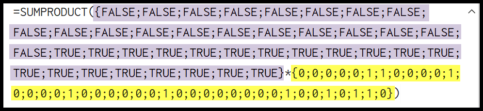
When we multiply both arrays with each other, we have a single array with 0 and 1. In this array, one (1) is for the value “Female” in the gender and 21-30 for the “Age Slab”.

In the end, SUMPRODUCT returns the sum by using this array. And this sum is the count of cells with the value “Female” in the gender column when you filter the 21-30 slab in the “Age Slab” column.