How to Get Quarter from a Date in Excel

Get Quarter by using ROUNDUP and MONTH Functions

Using a combination of ROUNDUP and MONTH is the best way to find the quarter of a date. It returns a quarter as a number (like 1, 2, 3, 4). Here’s the formula.

=ROUNDUP(MONTH(A1)/3,0)

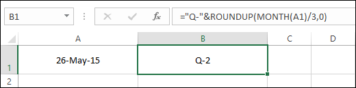
Here we are using 26 May 2018 as a date and the formula returns 2 in the result. You can use the below formula if you want to add a Q before the quarter number.

="Q-"&ROUNDUP(MONTH(A1)/3,0)

How This Formula Works

This formula works in three parts. In the first part, we used the MONTH function and referred to the date, which returns the month number.

After that, in the second part, we divided that month number by 3, which gives us a number with decimals.

At last, in the third part, we used the ROUNDUP function to round up that number with decimals, which gives us the actual quarter.

Here’s the real thing: You know there are 4 quarters and twelve months. Right? And if you divide all the month numbers by three (yes, just by 3), you’ll get something like the below.

And when you round them up, you’ll always get the quarter number for the month.

Get Quarter by using the Fiscal Calendar

In the above example, we have used a simple formula to have a quarter from a date, but sometimes you need to use a fiscal calendar.

What is a Fiscal Year?

A fiscal year (FY) is a 12-month period that a company or government uses for accounting purposes and preparing financial statements. A fiscal year may not be the same as a calendar year…

…learn more

And for a fiscal calendar quarter calculation, we need to use a different formula, and in this formula, we need to combine the CHOOSE and MONTH functions. Here’s the formula:

=CHOOSE(MONTH(A1),4,4,4,1,1,1,2,2,2,3,3,3)

(Here I’ve used the Indian fiscal year which starts on 1 April and ends on 31 March)

It returns 1 in the result, as the month is May, our year starts in April, and May is the second month of the year, which comes under the first quarter.

How This Formula Works

Here we have combined two different functions and it works in two parts.

In the first part, we have used the MONTH function to get the month number from the date and here it returns 5.

After that, in the second part, we have used the CHOOSE function to get a number according to the month number returned by the MONTH function.

If you look, in the CHOOSE function, we have specified 12 different numbers (4,4,4,1,1,1,2,2,2,3,3,3), so when MONTH returns a number, CHOOSE returns the number at that position in this list. Here’s the deal:

For the first three numbers, we have 4, which means if it returns 1, 2, or 3 (Jan-Mar), we will get 4, and for the next three months, we will get 1 (that’s because our fiscal year starts in April).

If your fiscal year starts in another month, you can change the numbers in CHOOSE, or use the following formula, where 4 is the first month of the fiscal year (change it to 7 for a year that starts in July, or 10 for October):

=ROUNDUP((MOD(MONTH(A1)-4,12)+1)/3,0)

MOD turns the month into its position in the fiscal year (April = 1, March = 12), and the rest works like the first formula. For 31-Mar-2018, it returns 4, and for 1-Apr-2018, it returns 1.

Use the CEILING Function to Get the Quarter

Like the ROUNDUP, it also rounds up the month number divided by 3 to the nearest integer to find the quarter.

=CEILING(MONTH(A1)/3, 1)

Like all the other formulas we have discussed, it helps you get the quarter of the year a date falls into.

First, it finds the month number of the date. Then, it divides this month’s number by 3. Finally, the CEILING function rounds up the result to the nearest whole number, the quarter.

Use QUOTIENT and IF to Check Quarter

QUOTIENT can divide one number by another and then give you the result without any remainder. Subtract 1 from the month number, divide it by 3 with QUOTIENT, and add 1 to get the quarter:

=QUOTIENT(MONTH(A1)-1,3)+1

Or, if you prefer to check the month with conditions, below is the formula that you can use with nested IF functions.

=IF(MONTH(A1)<=3, 1, IF(MONTH(A1)<=6, 2, IF(MONTH(A1)<=9, 3, 4)))

This formula checks the quarter of the year for a date in cell A1. It checks the month of the date: if it’s March or before, it returns 1, indicating the first quarter. If it’s June or before, it returns 2 for the second quarter.

If it’s September or before, it returns 3 for the third quarter. Otherwise, it returns 4 for the fourth quarter.

Get Start Date of the Quarter from a Date

Let’s forget about the quarter number and get the starting date of the quarter.

That means if we have the date 26-May-2018, instead of having quarter number 2, we can have 01-Apr-2018, which is the starting date of the first month of the quarter. Here’s the formula which we need to use:

=DATE(YEAR(A1),FLOOR(MONTH(A1)-1,3)+1,1)

When you enter this formula, it simply returns the starting date of the quarter.

How This Formula Works

This formula is made up of four different parts which give you the starting date of a quarter.

In the first part, we have used the MONTH function, which returns the month number for the date.

So when MONTH returns 5 as the month number (and we subtract one from it to get 4), in the second part, FLOOR rounds it down to 3, and then we add one to it, so we get 4, which is the first month (April) of the same quarter.

After that, in the third part, we used the YEAR function to get the year from the actual date. And in the fourth part, we have simply used the DATE function to create a date by combining the values that come from the first three parts (the year, the first month of the quarter and day 1).

Get End Date of a Quarter from a Date

OK, so you need the end date of a quarter instead of the start date or the number, and for this, the formula which we can use is:

=DATE(YEAR(A2),((INT((MONTH(A2)-1)/3)+1)*3)+1,1)-1

For 26-May-18, it returns 30-Jun-18, which is the last date of the quarter.

If you prefer a shorter formula, EOMONTH can do the same. MOD works out how many months are left to the end of the quarter, and EOMONTH returns the last day of that month:

=EOMONTH(A1,MOD(3-MONTH(A1),3))

EOMONTH returns a date serial number, so apply a date format to the cell to see it as a date.

How This Formula Works

In this formula, we have four different parts.

In the first part, we have combined the INT and MONTH functions. MONTH returns the month number of the date, we subtract 1 from it, and then divide it by 3. After that, INT rounds it down to the nearest integer, and we add 1 to it to get the quarter number.

In the end, we multiplied it by 3 to get 6 (June), which is the end month of the quarter, and then added 1 to it.

In simple words, this part of the formula simply converts the month of the actual date to the next quarter’s first month.

In the second part, we used the YEAR function to get the year from the actual date.

After that, in the third part, we simply used 1 as the day to complete the date with the DATE function.

Sorry! One more thing. In the fourth part, we subtract 1 from the entire formula, so that we get the last date of the quarter instead of the first date of the next quarter. For a date in December, the month becomes 13, and DATE moves it to January of the next year, so the result is still 31 December.

Convert a Date into a Quarter using VBA Code

Here we are using a VBA code to simply convert a date into its quarter number. Here’s the code:

Sub convert2Quarter()
Dim Rng As Range
For Each Rng In Selection
If IsDate(Rng.Value) = True Then
Rng.Value = DatePart("q", Rng.Value)
Rng.NumberFormat = "General"
End If
Next Rng
End Sub

To use this code all you need to do is to add it to your VB editor.

And then simply select the cells where you need to convert a date into a quarter number and finally run this code.

Here’s how this code works…

When you run this code, first it checks whether the cell has a date or not, and if it’s a date, then it converts it into the quarter number. We have used two different VBA functions here:

1. ISDATE: To check whether the cell has a date.
2. DATEPART: To convert a date into a quarter.

Check this out: Macro Codes for VBA New Comers | What is VBA in Excel

Create a Custom Function for Quarter

Function GetQuarterFromDate(rng As Date) As String
    Dim monthNumber As Integer
    monthNumber = Month(rng)
    
    Select Case monthNumber
        Case 1 To 3
            GetQuarterFromDate = "Q1"
        Case 4 To 6
            GetQuarterFromDate = "Q2"
        Case 7 To 9
            GetQuarterFromDate = "Q3"
        Case 10 To 12
            GetQuarterFromDate = "Q4"
    End Select
End Function

Put this function in a standard module (Insert ➜ Module) in the VBA editor, and then use it in a cell like any other function, like =GetQuarterFromDate(A1). It returns the quarter as text, like “Q2”.

Get Quarter and Year Together

When your dates cover more than one year, a quarter number alone isn’t enough, as Q2 of 2018 and Q2 of 2019 look the same. Add the year to the result with the following formula, which returns Q2-2018 for 26-May-2018:

="Q"&ROUNDUP(MONTH(A1)/3,0)&"-"&YEAR(A1)

And if the cell might be blank, wrap the formula in IF. Otherwise, a blank cell is read as day 0 and you get a quarter for it:

=IF(A1="","",ROUNDUP(MONTH(A1)/3,0))

Group Dates by Quarter in a Pivot Table

If you only need totals by quarter, you don’t need a formula at all. Add the date field to the Rows area of a pivot table, right-click any date, select Group, and then select Quarters (and Years, if your data covers more than one year). In Power Query, you can add the quarter with Add Column ➜ Date ➜ Quarter ➜ Quarter of Year.

Frequently Asked Questions

=YEAR(A1)+(MONTH(A1)>=4)