VLOOKUP is the easiest way to match two columns with each other and get result on which values match. In the below example, we have two lists of names. In the first, we have 20 names and in the second we have 10 names.

Now you need to compare both columns with each other using VLOOKUP.
Comparing the First Column with the Second Column
You need to follow below steps:
- In column B, next to column A. In cell B2, enter the VLOOKUP.
- In the lookup_value, refer to the cell A2.
- For table_array, refer to the range D1:D11; to freeze the range, you can use a dollar sign ($D$1:$D11).
- Type 1 in the column_index_num.
- And in the range_index, enter 0 and close the function.

Now, hit enter to get the result and then drop down the formula up to the last name. As you can see, four values in the column match the names in the second column.
= VLOOKUP(A2,$D$1:$D$11,1,0))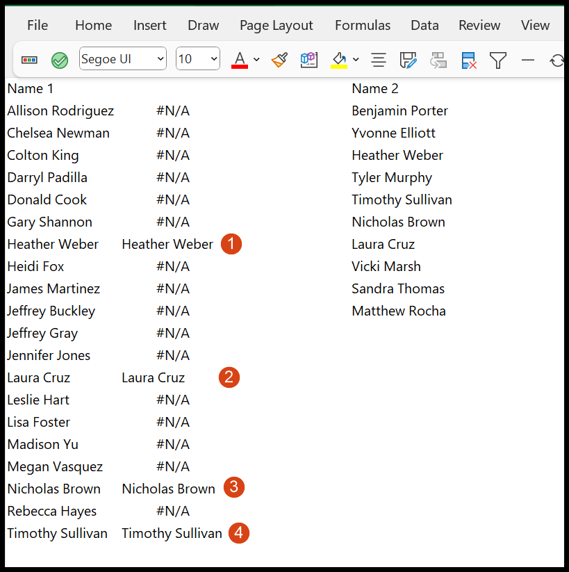
And if you want to compare the second column with the first column, you can use the same formula.
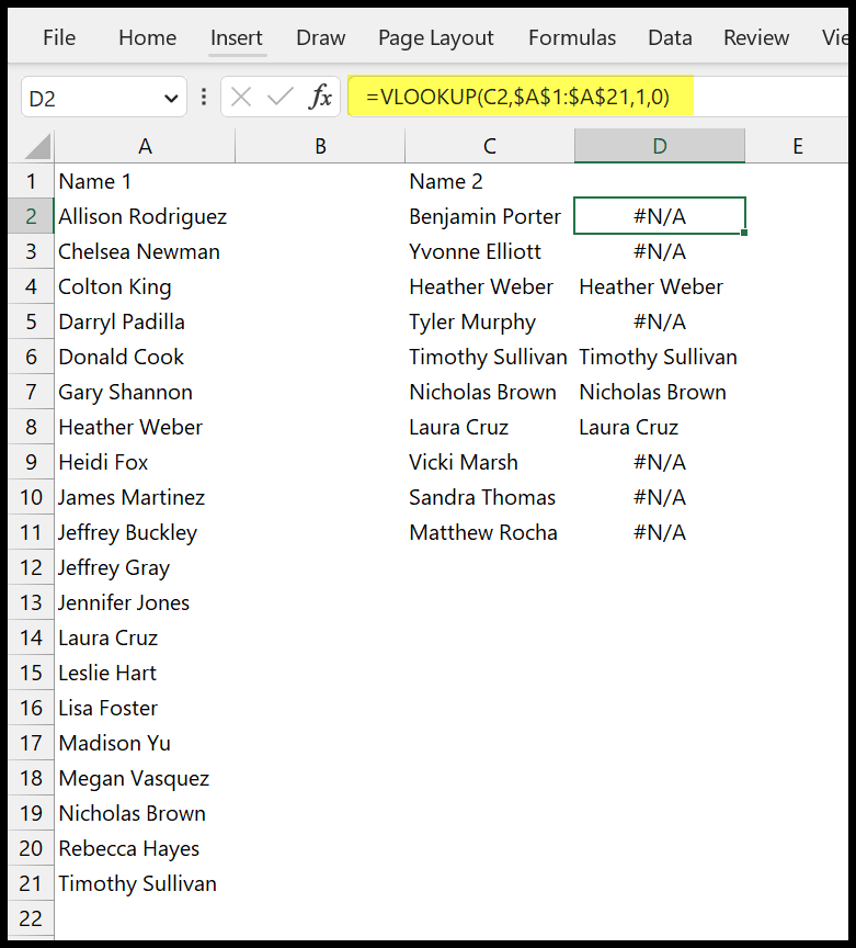
=VLOOKUP(C2,$A$1:$A$21,1,0)You need to freeze the range by using the dollar sign ($) in the table_array so that when you drag the formula down, it won’t move the table_array along with it.
Getting a Meaningful Answer to the Result
As you can see, we have an #N/A error for the values not in the second column. Now to convert this error to something meaningful, you can use the below formula:
=IF(ISERROR(VLOOKUP(A2,$D$1:$D$11,1,0)),"Not Available","Available")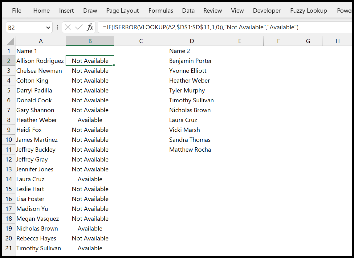
This formula uses ISERROR to check the error and then uses IF. If there’s an error, it returns a value you have specified; otherwise, another value you have set.