

Select the range, then go to Home → Conditional Formatting → Highlight Cells Rules → Duplicate Values, choose a format and click OK. Every value that appears more than once is highlighted, including its first occurrence.
To flag the opposite, change the first drop-down in that dialog from Duplicate to Unique. This highlights the values that appear only once.
To highlight values that appear three or more times, select the range starting at A1, go to Home → Conditional Formatting → New Rule → Use a formula to determine which cells to format and enter =COUNTIF($A$1:$E$7,A1)>2. To read the count from a cell instead, replace >2 with >=$G$3.
To leave the first occurrence plain and mark only the repeats, select one column starting at A2 and use =COUNTIF($A$2:A2,A2)>1. Because the range expands as it goes down, each row counts only itself and the rows above it.
The check ignores case, so Apple and APPLE count as duplicates. A trailing space has the opposite effect: two values that look the same won’t match, so clean them with =TRIM(A2) first. In a formula rule, the relative reference must point at the top-left cell of your selection, or the highlights land on the wrong cells.
Using conditional formatting is the best way to quickly highlight duplicate values in Excel. And in this tutorial, we will learn these steps in detail.
Steps to Highlight the Duplicates
- Select the range of cells where you have the data.

- Afterward, go to Home > Conditional Formatting > Highlight Cells Rules > Duplicate Values.

- Now, you have a dialog box to specify the color you want to apply to the cells with the duplicate values.

- And the moment you click OK, you have all the duplicate cells highlighted in red.

As I said, it’s the quickest way to highlight and find duplicate values from a range of cells. It’s a pre-built rule in conditional formatting that you can use. From the same option, you can find unique values as well. You can change it from the drop-down (Duplicate or Unique).
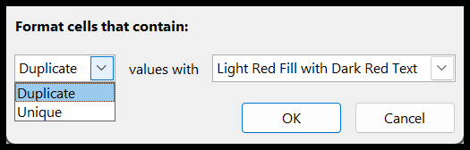
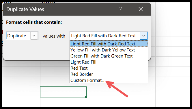
And you can also use different formatting if you want. There are six pre-defined formats that you can use, or you can choose your own formatting with the Custom Format option.
Highlighting Triplicates with Conditional Formatting
You can also highlight values which are triplicates, and not only triplicates but all the values that appear 3 or more times in the data. We don’t have a pre-defined rule for this, but we can create a custom rule using a formula.
- Select the data from where you want to highlight values.
- Go to Home > Conditional Formatting > New Rule.
- And then, click on “Use a formula to determine which cells to format”.
- Enter the formula (=COUNTIF($A$1:$E$7,A1)>2), and click on the Format button to choose the cell formatting.
- In the end, click OK (or hit Enter) to apply the rule.
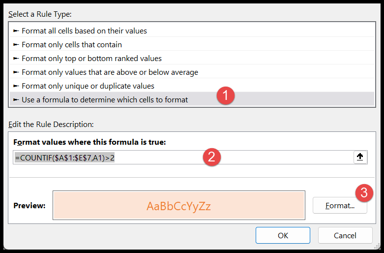
And the moment you hit Enter, it highlights all the values that occur more than twice.
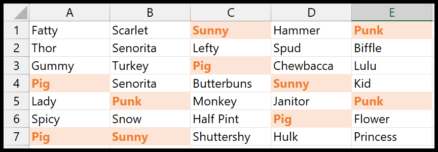
In the above example, you can see we have highlighted all the values that occur more than 2 times in the entire data. And the formula which we have used is quite simple.
=COUNTIF($A$1:$E$7,A1)>2
In this formula, we have used COUNTIF to count each cell’s value in the entire range. And if the count of the value is more than 2, it returns TRUE in the result. And when it’s true, it applies the conditional formatting rule.
Here’s another example where we have used a reference to cell G3 instead of the number 2. Now the rule is dynamic, and when you change the value in the cell, it uses that number to test the occurrence of the value in the range.
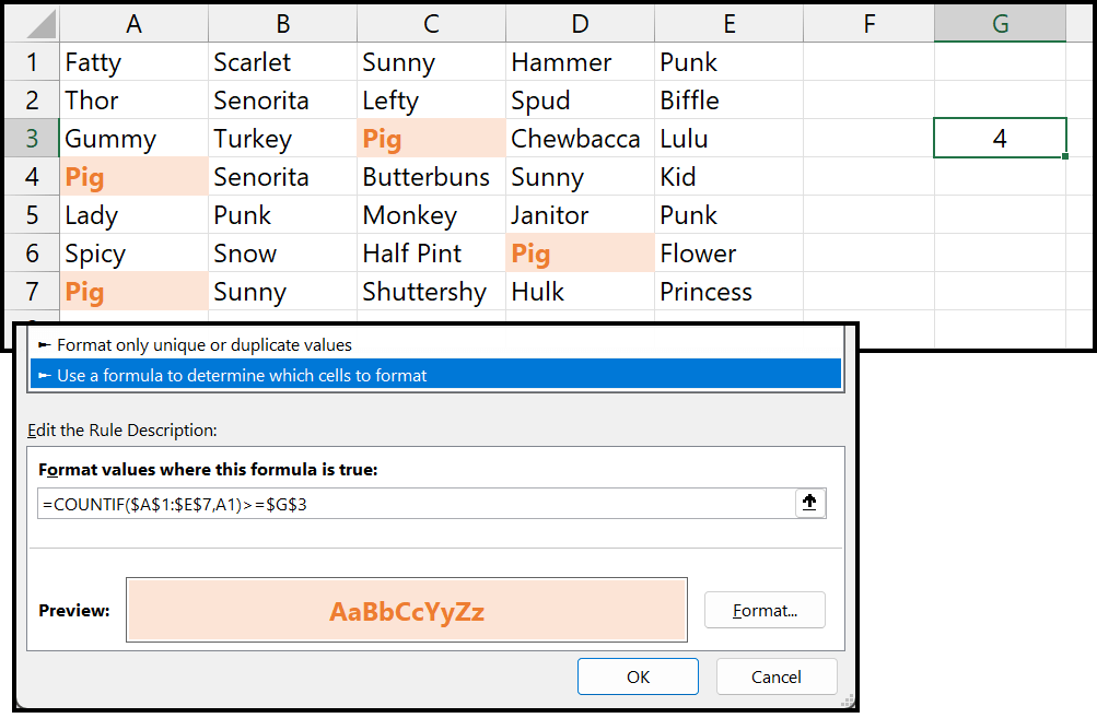
The best part of using conditional formatting to find and highlight duplicates is it’s quick and pre-defined. You don’t need to put any extra effort into using it.
Keep in mind that the Duplicate Values rule isn’t case-sensitive, so “Apple” and “apple” count as duplicates. And a value with an extra space at the end isn’t a duplicate of the same value without the space.
Highlight Duplicates but Skip the First Occurrence
The pre-built rule highlights every copy of a value, including the first one. If you only want to highlight the second, third and later copies, select the column (for example, A1:A20) and use this formula in a new rule:
=COUNTIF($A$1:A1,A1)>1
The range starts at $A$1 and grows one row at a time, so the formula only counts the cells above and including the current one. The first time a value appears, the count is 1, and it’s not highlighted.
Highlight Duplicate Rows
To highlight rows where the values in two columns are both repeated (like the same name and the same city), select the data, say A1:B20, and use COUNTIFS in a new rule:
=COUNTIFS($A$1:$A$20,$A1,$B$1:$B$20,$B1)>1
The $ before the column letters keeps the formula on columns A and B, so the whole row gets the color when the pair of values appears more than once.
Frequently Asked Questions
How do I remove the duplicate highlighting?
Select the range and go to Home > Conditional Formatting > Clear Rules > Clear Rules from Selected Cells. The values stay as they are; only the formatting rule is removed.
Why are numbers that look the same not highlighted?
They’re probably different underneath: one may be a number stored as text, have hidden decimals, or have an extra space. Check them with =ISTEXT(A1) or =LEN(A1).
Can I delete the duplicates after highlighting them?
Yes. Use Data > Remove Duplicates to delete them, or filter the column by cell color to see only the highlighted cells.
Written by
Puneet Gogia
Microsoft MVP — Excel · Founder, Excel Champs
Twelve years of teaching Excel, and a decade before that using it as a data analyst. Every tutorial here is written from a file I actually built.