Find and Highlight Duplicates in Excel using Conditional Formatting

Using conditional formatting is the best way to quickly highlight duplicate values in Excel. And in this tutorial, we will learn these steps in detail.

Steps to Highlight the Duplicates

1. Select the range of cells where you have the data.
   
2. Afterward, go to Home > Conditional Formatting > Highlight Cells Rules > Duplicate Values.
   
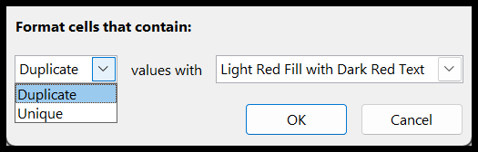
3. Now, you have a dialog box to specify the color you want to apply the cells with the duplicate values.
   
4. And the moment you click OK, you have all the cells highlighted with the red color.
   

As I said, it’s the quickest way to highlight and find duplicate values from a range of cells. It’s the pre-built rule in conditional formatting which you can use. From the same option, you can find unique values as well. You can change it from the drop-down.

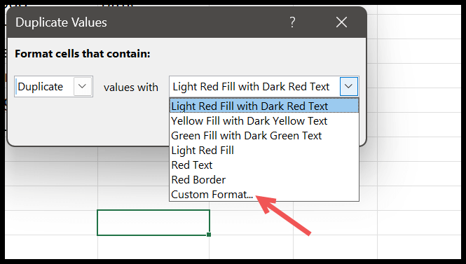
And you can also use the different formatting if you want. There are six pre-defined formatting that you can use, or you can choose formatting from the custom formatting option.

Highlighting Triplicates with Conditional Formatting

You can also use highlight values which are triplicates, not only triplicates but all the values more than 3 times in the data. We don’t have a pre-defined rule, but we can create a custom rule using a formula.

1. Select the data from where you want to highlight values.
2. Go to Home > Conditional Formatting > New Rule.
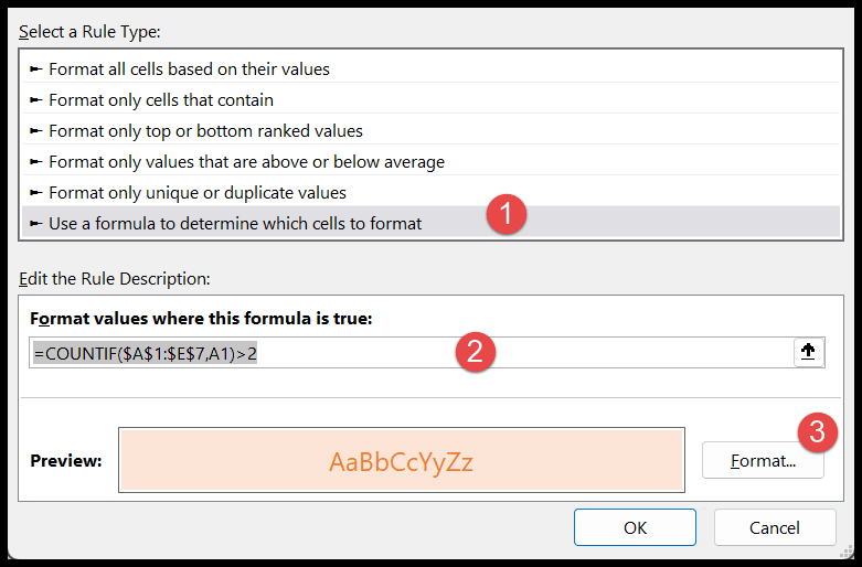
3. And then, click on “Use a formula to determine which cells to format”.
4. Enter the formula (=COUNTIF($A$1:$E$7,A1)>2), and click on the format button to apply the cell formatting.
5. In the end, hit enter to apply the rule.

And the moment you hit enter, it highlights all the where you have occurred more than twice.

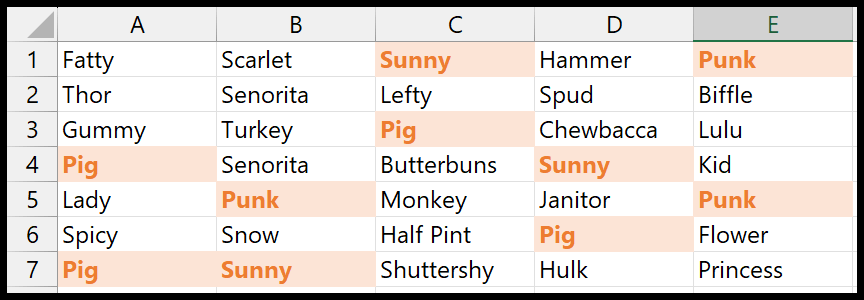
In the above example, you can see we have all the values whose occurrence is more than 2 in the entire data. And the formula which we have used is quite simple.

=COUNTIF($A$1:$E$7,A1)>2

In this formula, we have used COUNTIF to count each cell’s value with the entire range. And if the count of the values is more than 2, it returns TRUE in the result. And when it’s true, it applies the conditional formatting rule.

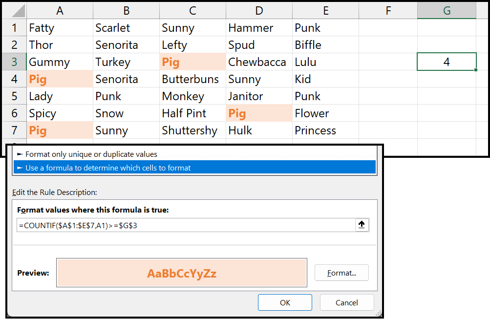
Here’s another example where we have used a cell reference to cell G3. Now the rule is dynamic, and when you change the value in the cell, it uses that number to test the occurrence of the value in the range.

The best part of using conditional formatting to find and highlight duplicates is it’s quick and pre-defined. You don’t need to put any extra effort into using it.