Apply Conditional Formatting Based on Another Column in Excel

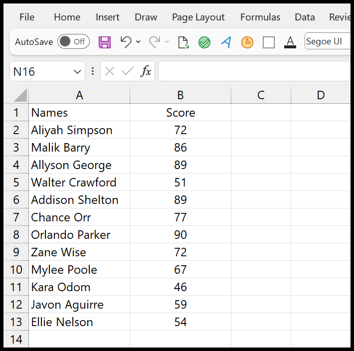
In Excel, you can apply conditional formatting based on another column. For example, below, you have a list of students with their scores, and you want to highlight the names of students who scored above 75.

Now here, you need to apply conditional formatting, which applies color to column A (Names) based on the values in column B (Score).

Steps to Apply Conditional Formatting Based on Another Column

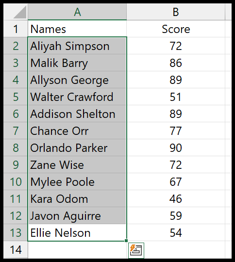
1. First, select the names column by leaving the column name.
   
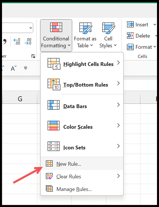
2. Afterward, go to the Home Tab > Conditional Formatting > New Rule.
   
3. Next, in the new rule dialog box, click “Use a Formula to determine which cell to format”.
   
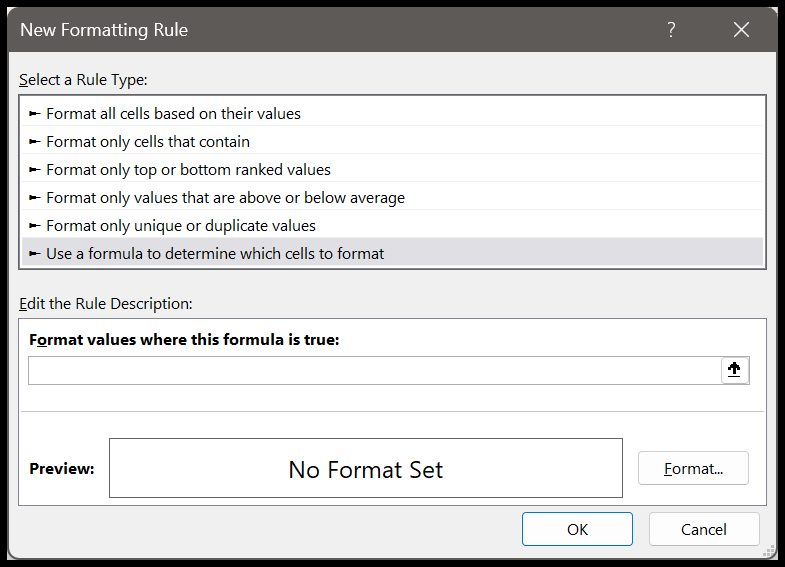
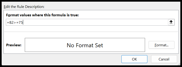
4. Now, in the ‘Format value where this formula is true” dialog box, enter this formula =$B2>=75.
   
5. From here, click on the “Format…” button to specify the cell formatting you want to apply to the student’s name cell, and in the end, click OK to save the rule.
   
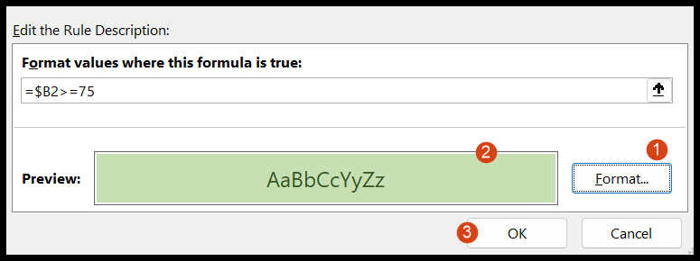
6. In the end, click OK to close the conditional formatting rules manager.

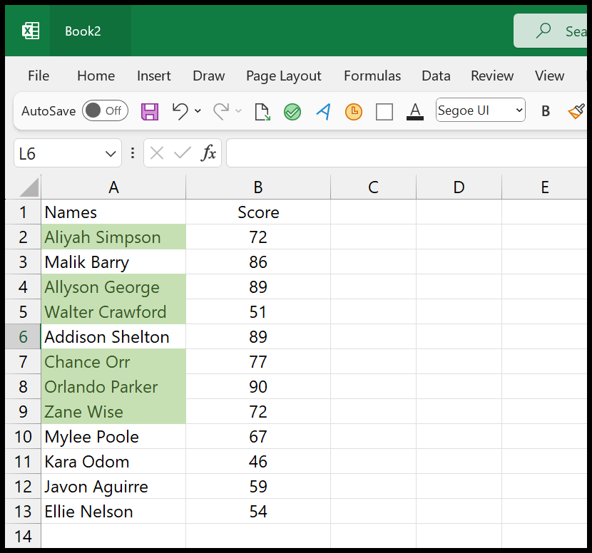
And the moment you click OK, it will highlight all the names of the students whose score is greater than 75 in the score column.

Using an Excel Table

Once you apply the conditional formatting and when you update new data in the list, Excel will not extend the conditional formatting to the new entry.

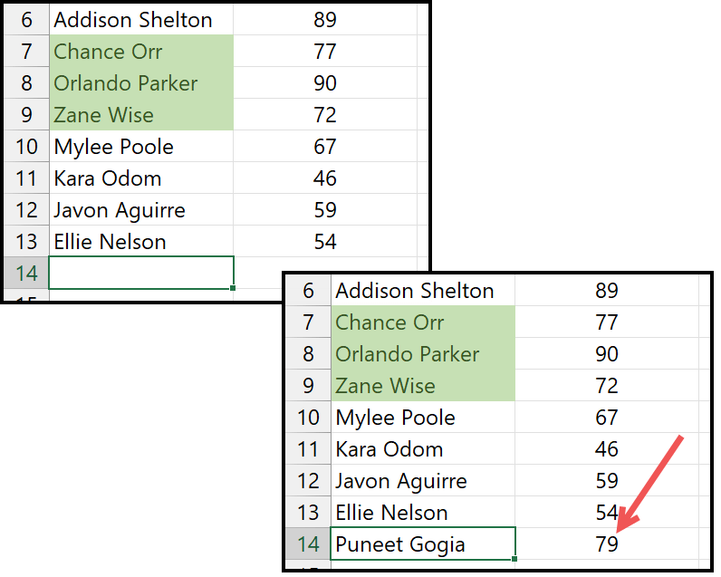
The best solution to this problem is to use an Excel table on the data. Once you apply the table (Ctrl + T) and then enter a new data entry to the list with the score, apply conditional formatting to it.

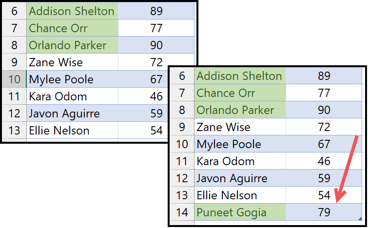
Using an Excel table make your conditional formatting rule dynamic, which extends itself when you enter a new value in the data.