

Select the numbers only, without headers or totals, then go to Home → Conditional Formatting → Color Scales and pick a scale. The first one, Green – Yellow – Red Color Scale, shades the highest values green and the lowest red, with everything else graded in between.
To change the colours or the break points, go to Home → Conditional Formatting → Manage Rules → Edit Rule. Choose 2-Color Scale or 3-Color Scale and set the minimum, midpoint and maximum as Number, Percent or Percentile. Fixed numbers keep the same colour meaning the same value from one month’s sheet to the next.
To show only the colours, select the range, press Ctrl + 1, go to Number → Custom and type ;;; in Type. The values stay in the cells, so formulas and the formula bar still see them.
In a pivot table, select one value cell, apply the colour scale, then open Manage Rules → Edit Rule and set Apply Rule To to the last option, All cells showing “Sum of Sales” values for “Region” and “Month” (with your own field names). The scale then covers every value cell after a refresh or filter change and leaves subtotals and grand totals out.
If nearly every cell comes out the same colour, a total is inside the range. It is the largest number, so it takes the top colour and squeezes the rest into the bottom of the scale: remove the total row or column from Applies to in Manage Rules. Numbers stored as text get no colour at all, so convert them before you read the map.
Visuals are always easier to understand compared to values. Even in Excel, when you use a chart (advanced or basic), it becomes easy for the user to understand the data.
But we can’t go this way every time, as most of the time, we need to present our data in tables or in other report formats.
To deal with this kind of situation in Excel, I have found that a heat map is the best solution. It helps us present data with a visual effect and without changing the actual data structure.
What is a HEAT MAP in Excel?
In Excel, a Heat Map is a presentation of data that uses a color shade on each cell in a range, in a comparative way, so a user can understand it easily. It looks like a map with different colors ranging from dark to light to represent the weightage of the value in the cell.
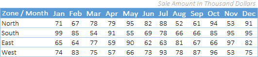
Below is an example of a simple heat map where we have zone-wise and month-wise data, and every cell with a sales value has a color shade applied to it.

And this color shade helps us to quickly compare values in the cells with each other. The cell with the highest value is green, the cell with the lowest value is red, and the cells in the middle are yellow.
All the values between the highest value and the lowest value get a color shade according to where they fall in that range. You can’t really create a heat map like this manually, because picking a color for every cell according to its value isn’t practical, especially when the values change.
Now the point is: what are the possible ways to create a heat map in Excel? And if you ask me, there are more than three. So in this post, I’ll be sharing all the possible ways to create a heat map in Excel.
When you take a printout of a heat map on paper it looks really nasty especially when you are using a black and white printer. All the shades only have black and white color which is not easy to understand for anyone.
Create a Heat Map in Excel using Conditional Formatting
If you don’t want to put in extra effort and want to save time, you can create a simple heat map by using conditional formatting. I’m using the same data as a sample (DOWNLOAD LINK) here, which I showed you at the start of this post.
To create a heat map in Excel you need to follow the below steps:
- First of all, select the data on which you want to apply a heat map (here, you need to select all the cells where you have sales values).
- After that, go to Home Tab ➜ Styles ➜ Conditional Formatting.
- In conditional formatting options, select Color Scales. (You have 12 different color scales to choose from.)

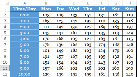
- Once you select an option, all the cells will get a color shade according to their value, and you’ll get a heat map like below.

- And if you want to hide the values and only show the color shades, you can use custom formatting for this.
- For this, first of all, select the heat map data and open the Format Cells dialog (Ctrl + 1).
- Now, in the Number tab, go to Custom, enter ;;; and in the end, click OK.

- Once you click OK, all the numbers will be hidden in the cells. Well, they are still in the cells, just hidden.

Steps to add a Heat Map in a Pivot Table
You can also use a heat map in a pivot table by applying conditional formatting. These are the steps to follow:
- Select any of the cells in the pivot table.
- Go to Home Tab ➜ Styles ➜ Conditional Formatting.
- In conditional formatting options, select Color Scales.

When you select a single cell, Excel applies the color scale to that cell only. Click the Formatting Options button that appears next to it and choose All cells showing “Sum of …” values (the name of your value field), so the whole pivot table gets the heat map and keeps it when you refresh.
Further, if you want to hide numbers (which I don’t recommend), please follow these simple steps.
- Select any of the cells in the pivot table.
- Go to PivotTable Analyze Tab ➜ Active Field ➜ Field Settings.

- Click on Number Format.
- In the Number tab, go to Custom and enter ;;; in Type.
- Click OK.
You can download this sample file from here to learn how we can use a slicer with a heat map pivot.
Steps to Create a Dynamic Heat Map in Excel
You can create a dynamic heat map if you want to hide/show it according to your need.
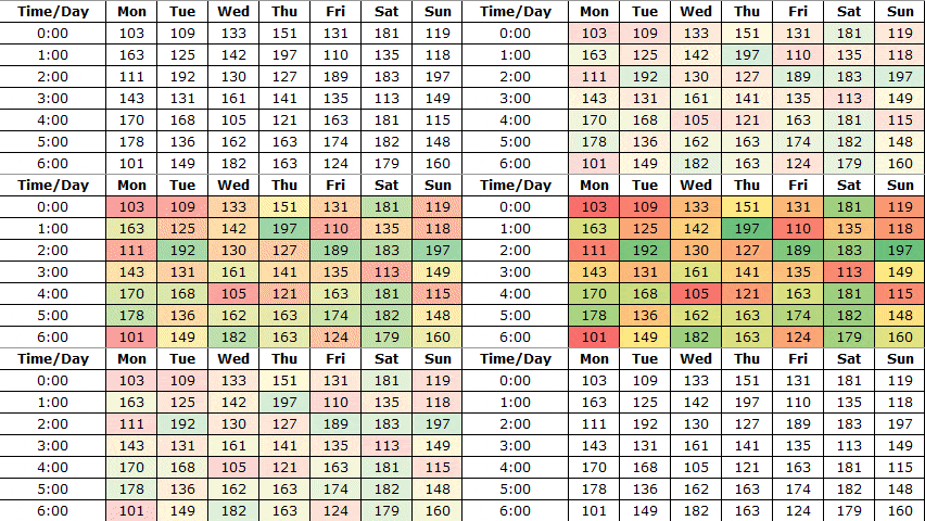
Below is the table we have used to create a dynamic heat map.
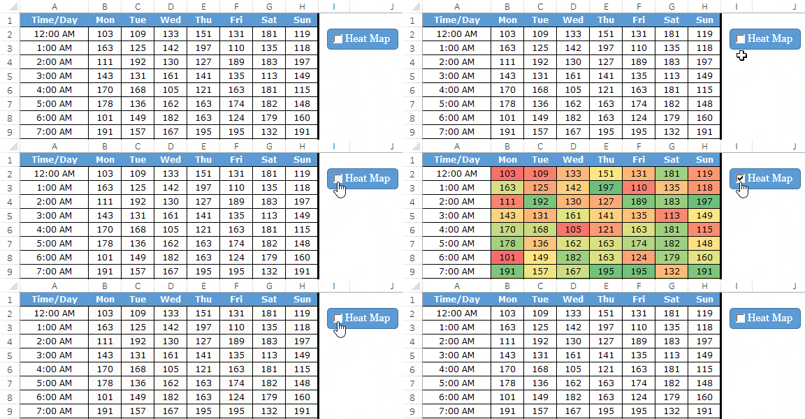
And these are the things we need to incorporate.
- Option to switch between heat-map and numbers.
- Auto-update the table with the heat map when you add new data.
Here’s how to do this:

Now you have a dynamic heat map that you can control with a check box.
And if you want to hide the numbers when you tick the checkbox, you need to create a separate conditional formatting rule. Here’s how to do this:
- Open conditional formatting new rule dialog box.
- Select “Use a formula to determine which cells to format” and enter the below formula.

- =IF($K$1=TRUE,TRUE,FALSE)
- Now, specify custom number formatting.
After applying all the above customization, you will get a dynamic heat map. (The formula can also be just a reference to $K$1, as the linked cell already holds TRUE or FALSE.)
Customize the Colors of a Heat Map
The built-in color scales may not fit your data. For example, for costs or errors, a high value is bad, so you may want red for the highest value. Here’s how to change it.
- First of all, select the heat map range and go to Home ➜ Conditional Formatting ➜ Manage Rules.
- After that, select the color scale rule and click Edit Rule.
- Next, choose 2-Color Scale or 3-Color Scale, and pick the color for Minimum, Midpoint and Maximum.
- You can also change the Type from Lowest/Highest Value to Number, Percent or Percentile, like a fixed target of 100 for the midpoint.
- In the end, click OK twice.
One more tip: when you apply the color scale to the whole table, each cell is compared with all the other cells. If you want to compare values within each row (like each zone across the months), apply the color scale to each row separately.
For a black and white printout, use a single-color 2-color scale (like white to dark grey) instead of red-yellow-green, so the shades still go from light to dark on paper.
More Information
These are some links to help you out while choosing your favorite color scheme.
Sample File
Download this sample from here to learn more.
Conclusion
Imagine you are looking at a large data set: it’s really hard to identify the lower or higher values, but if you have a heat map, it’s easy to identify them.
You can use different color schemes to illustrate a heat map. And if you can put in some extra effort, a dynamic heat map is the best. I hope this tip will help you get better at Excel, and now tell me one thing.
Do you think a heat map can be helpful for you in your work?
Share your views with me in the comment section; I’d love to hear from you. And, please don’t forget to share this tip with your friends.
Frequently Asked Questions
How do I reverse the colors of a heat map?
Pick the opposite preset from Color Scales (red for high values instead of green), or edit the rule in Manage Rules and swap the Minimum and Maximum colors.
Why is my heat map all one color?
Usually one value (like a grand total in the range) is much bigger than the rest, so all the other cells look alike. Leave totals out of the selection, or set the Maximum type to Percentile.
Can a heat map use text cells?
No. Color scales only work on numbers, so cells with text (or numbers stored as text) stay without color. Convert those values to numbers first.
Thanks for tutorial, much appreciated !
Thank you for teaching how to use heat map.
Hi Puneet,
Simple but very useful tips and tricks…
Beautiful option for formatting through colour from value.
Please share some VBA tutorials..
Here you go…
https://excelchamps.com/vba/
Thank you so much for sharing! I have been following you for awhile and your blogs has helped my work greatly! Thank you!!!
You’re welcome.
I really like your web site’s content but these pop-up messages are so incredibly annoying that I will not be back. I think they’re called “exit intent” popups. They are horrible. By the time I scrolled down 1/2 I was bombarded with no less than 3 pop-ups: on on the bottom-right, one even larger one on the bottom-left covering a lot of content, and then the entire screen became a pop-up. If these pop-up things arent smart enough to know that I have already signed up for a newsletter then what good are they? Isnt that what we’re wanting to learn – how to be smarter with technology? I hope you’ll consider removing it but I understand that you shouldnt just for me.
Lesson learned
Nice
Thanks for your words. 🙂
Thank you PG, for sharing these tips on creating an awesome Excel Heat Map Template. It was very interesting, insightful, and something I’ll be using in future.
Sincerely,
Leonardo “List Legend” LaVito
Thanks Leo LaVito for your words.