One of the best ways to become an advanced pivot table user and use Excel for data analysis is by using calculated items and calculated fields in a pivot table.
Using formulas in a pivot table or custom calculation which don’t exist in the source data but work like other fields.
In simple words, these are the calculations within the pivot table. In the below example, you can see a pivot table with a calculated field which is calculating the average selling price. On the other hand, source data doesn’t have any type of field like this.

Pivot Tables are one of the INTERMEDIATE EXCEL SKILLS.
Calculated Field in a Pivot Table
In the Excel pivot table, the calculated field is like all other fields of your pivot table, but they don’t exist in the source data. But they are created by using formulas in the pivot table. Follow these simple steps to insert the calculated field in a pivot table.
- First of all, you need a simple pivot table to add a Calculated Field.

- Just click on any of the fields in your pivot table. You will see a pivot table option in your ribbon which further having further two options (Analyze & Design) Click on the analyze option, then on Fields, Items, & Sets. You will further get a list of options, just click on the calculated field.

- After clicking the calculated field, you will get a pop-up menu, just like below. This popup menu comes with two input options (name & formula) & a selection option.

- Name: Name of the calculated Field which will show in your pivot table.
- Formula: An input option to insert formula for calculated field.
- Fields: A drop down option to select other fields from source data to calculate a new field.
Calculated Items in a Pivot Table
Calculated items are like all other items of your pivot table, but the difference is that they are not in existence in your source data. They are just created by using a formula. You can edit, change or delete calculated Items as per your requirement.
- Just click on any of the items in your pivot table. You will see a pivot table option on your ribbon having further two options (Analyze & Design).
- Click on the Analyze, then on Fields, Items, & Sets.
- You will further get a list of options, just click on Calculated Item.

- After clicking the calculated item, you will get a pop-up menu, just like above. This popup menu comes with two input options (Name & Formula) & two selection options (Field & Items).
- We had already discussed “Name, Formula & Fields” in calculated fields.
- Items: To select the items for calculation.
- In this example, we are going to calculate the average selling price and, the formula will be = amount/quantity.
- In Fields option, select Amount & click on insert, then insert “/” division operator & insert quantity after that.
- Press OK.
- Now a new Field appears in your Pivot Table.

- Your new calculated field is created without any number format.

In this example, we are going to calculate the average for the first half of the year & for the 2nd half of the year. We just have to add the formula.
=average(jan, feb, mar, apr, may, jun)Now you have to calculate items in your pivot, showing an average of the first six months and the second six months of the year.
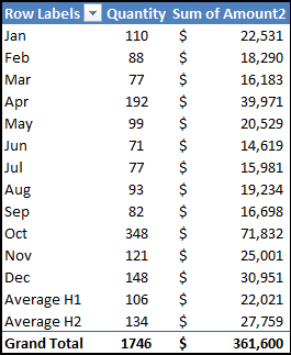
But wait a minute. What is this? Grand total is changed from 1506 & $311820 to 1746 & $361600.
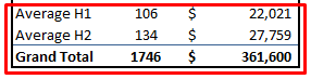
The reason behind this is, pivot table totals & subtotals include your calculated fields while the calculation of total and sub-total. So you need to filter your calculated items if you want to show the actual picture.
Things To Remember
- Don’t forget to remove 0 from the formula input option while inserting a formula for the calculation.
- You can only able to use formulas that don’t require cell references.
- You have to check whether calculated items are affecting your pivot results (Sub Totals and Grand Totals).
- Adjust the solve order are per your calculation requirement.
More on Pivot Tables
- Count Unique Values in a Pivot Table in Excel
- Add Ranks in Pivot Table in Excel
- Group Dates in a Pivot Table
⇠ Back to Pivot Table Tutorial
Very clear, concise directions which saves time
Thank you
Is it possible to find a difference between two columns in a pivot table?
Yes. Just write the formula that way. For example, if I want to calculate the difference between “target completion date” and “actual completion date”, the formula would be “=ACTUAL-TARGET”. In this instance, I would then have to format the new calculated column from date to number.
Hello Excel Champs, one question regarding calculated field, I’m trying to add a new field but formula is “X”column multiplied by TOTAL of “Y” Column, is that possible? To multiplied one field by the ColumnTOTAL of another field? Thanks!
Really helped a lot. Thank you!