

To count the weeks between two dates, subtract them and divide by seven: =(B1-A1)/7. From 01-Jan-2023 to 04-Jul-2023 that returns 25.86 weeks. Which formula you want depends on how you need the part-week handled.
For completed weeks only, wrap it in TRUNC: =TRUNC((B1-A1)/7) returns 25 and simply drops the remainder. To count a partial week as a full one, use =ROUNDUP((B1-A1)/7,0), which gives 26 — the right choice for billing periods or project scheduling.
And to show weeks and leftover days together, use =TRUNC((B1-A1)/7)&" weeks, "&MOD(B1-A1,7)&" days". Two things to know.
If the result appears as a date rather than a number, the cell has inherited a date format — press Ctrl+1 and set it to Number. And subtracting an earlier date from a later one gives a negative result rather than an error, so wrap it in ABS if your data might have the dates the wrong way round.
In Excel, you can use a formula to calculate the number of weeks between two dates. In this tutorial, we will learn to write this formula.

Here, in this example, we have two dates: the starting date is 01-Jan-2023, and the ending date is 04-Jul-2023.
Formula to Get Weeks Between Two Dates in Excel
- Enter TRUNC Function in a cell.
- Minus the starting date from the ending date.
- Divide it by 7 as there are 7 days in a week.
- Close the function and hit enter to get the result.
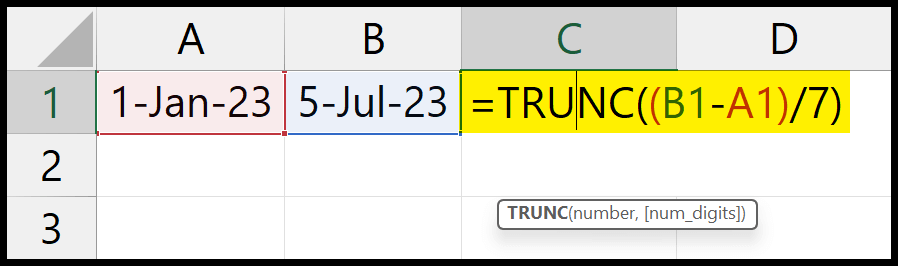
=TRUNC((B1-A1)/7)The moment you hit enter, it returns the count of complete weeks between the specified dates.
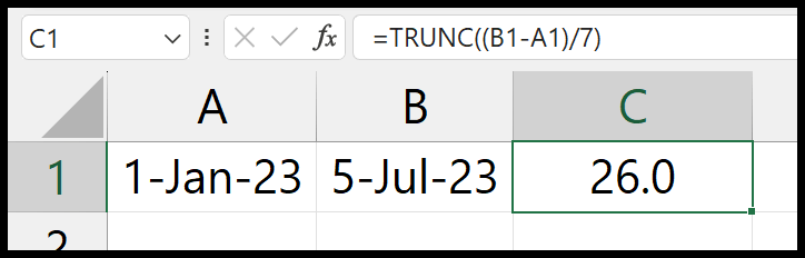
The way this formula works is simple: you subtract the starting date from the ending date to get the total number of days between the dates.
Then, divide that by 7 to get the number of weeks for those days. In the end, when you use the TRUNC function, it only returns the count of the complete weeks, ignoring the decimals.
But if you want to get the exact count of weeks, you can skip using the TRUNC function and use a simple formula like the following:
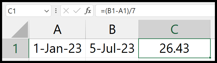
=(B1-A1)/7And if you want to round an incomplete week as a complete week, you can use the ROUNDUP function.
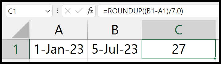
In the ROUNDUP, you can use the same formula in the number argument and 0 in the num_digit.
=ROUNDUP((B1-A1)/7,0)
nice