

In Excel, if you want to sort dates using the months, the best way is to create a helper column for the month numbers and then sort data based on those. And in this tutorial, we will learn the method in detail.

Let’s get started.
Steps to Sort Dates by Month
- First, in the second column (Column B) create a heading with the name “Month”.

- In cell B2, enter the MONTH function and refer to cell A2, where you have the date (formula below this list). Once you type it, hit Enter to get the result.
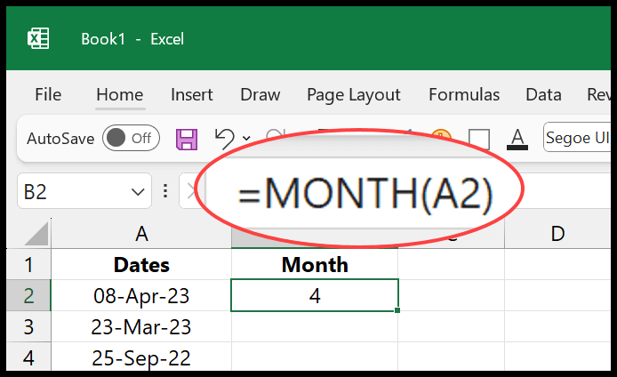
- After that, drag the formula down to the last cell of the column. You can double-click on the small green square at the bottom right of the cell. This will fill the formula down to the last cell.

- From here, you need to open the sorting option. Select the entire data and use the keyboard shortcut (Alt > A > S > S), or you can also go to Data > Sort & Filter > Sort to open the Sort dialog box.

- Next, from the “Sort by” drop-down, select the “Month” column. And from the “Order” drop-down, select “Smallest to Largest”.

- In the end, click OK to apply the sorting.
=MONTH(A2)
When you click OK, it sorts the data using the month column. And your dates get sorted by months, from January to December.
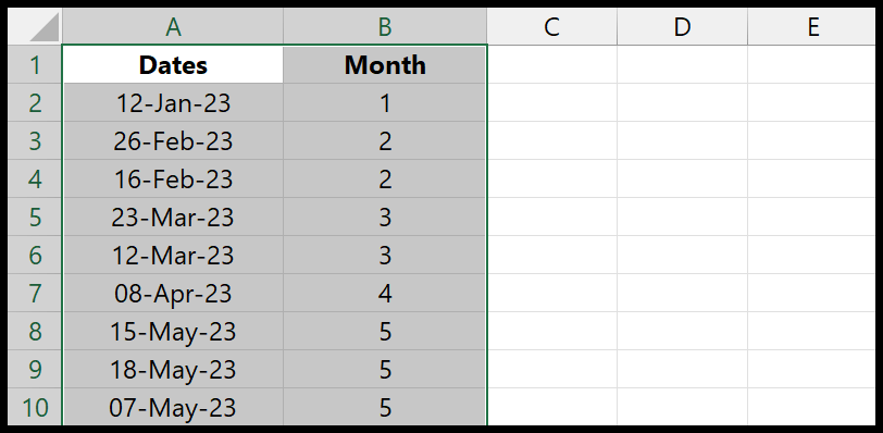
Using Month Names Instead of Numbers
Instead of using the month number, you can also use the month names and then sort the dates based on those month names. In the month column, enter the TEXT function to get the month name from the date.

=TEXT(A2,"MMMM")
From here, the next thing is to select the data and sort it using the month column. So, select the data and then use the keyboard shortcut (Alt > A > S > S) to open the SORT dialog box. Select the “Month” column from the “Sort By” in the SORT dialogue box.
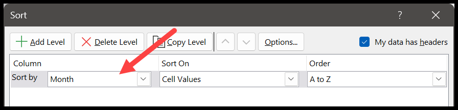
After that, from the “Order” drop-down, select “Custom List…”.
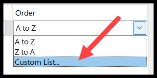
Selecting “Custom List…” will open a new dialog box from where you need to select the custom list of months to sort the data.
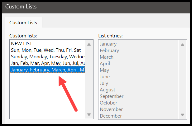
Note: If you don’t have the list of month names, you can learn to create it from this quick guide.
Finally, click OK to go back to the SORT dialog box and again OK to apply the sorting. And once you click OK, it sorts the data based on your month names in the month column.
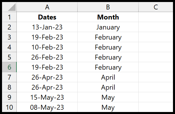
Sorting by the month name alphabetically (A to Z) won’t work, as it puts April first and September last. That’s why you need the custom list.
Sort by Month and Day (Ignoring the Year)
When you sort by the month number only, dates of the same month stay in their original order, and dates from different years get mixed. For a list like birthdays, where you want the month and then the day, use this helper formula instead and sort it from A to Z:
=TEXT(A2,"mmdd")
It returns 0315 for 15-Mar and 1231 for 31-Dec, so the text sorts in calendar order. If you want the month and then the year (like a timeline), sort by the date column itself, or use =TEXT(A2,”yyyymm”).
Sort by Month with a Formula
In Microsoft 365 and Excel 2021 or later, you don’t need a helper column. SORTBY returns the dates sorted by month in a new range, and the original data stays as it is:
=SORTBY(A2:A13,MONTH(A2:A13))
Make sure the range has no blank cells, as MONTH returns 1 for a blank cell, and it would be sorted with January.
Frequently Asked Questions
Why does MONTH return #VALUE! for some dates?
Those dates are stored as text that Excel can’t read as a date. Convert them first, for example with Data ➜ Text to Columns ➜ Finish, or with DATEVALUE.
Can I sort by month in a pivot table?
Yes. Group the date field by Months, and the pivot table sorts the months from January to December on its own.
Should I delete the helper column after sorting?
You can. The sort stays after you delete it. But if you keep it, you can sort again in one step whenever you add new dates.
Written by
Puneet Gogia
Microsoft MVP — Excel · Founder, Excel Champs
Twelve years of teaching Excel, and a decade before that using it as a data analyst. Every tutorial here is written from a file I actually built.