

Select the cells, then go to Home → Conditional Formatting → Highlight Cells Rules → Text that Contains. Type the word, for example priority, choose a format and click OK. Every cell with that word anywhere in it is highlighted, whatever its case.
For more control, use Conditional Formatting → New Rule → Use a formula to determine which cells to format with =ISNUMBER(SEARCH("priority",A2)), where A2 is the first cell of your selection. SEARCH ignores case; use =ISNUMBER(FIND("Priority",A2)) when case matters.
To change the word without editing the rule, type it in a cell such as C1 and use =AND($C$1<>"",ISNUMBER(SEARCH($C$1,A2))). The $C$1<>"" part stops every cell lighting up while C1 is empty, because a search for an empty string always matches.
To colour the whole row, select the full table and lock the column: =ISNUMBER(SEARCH("priority",$A2)). COUNTIF works too, but it needs wildcards to match part of a cell: =COUNTIF(A2,"*priority*")>0. Without the asterisks it only matches cells that hold exactly that word and nothing else.
If nothing highlights, retype the quote marks in Excel: curly quotes pasted from a web page make the rule fail. Also note that * and ? act as wildcards in SEARCH and COUNTIF, so put a tilde before them (~?) to find the literal character.
Let’s say you work in a sales department and have an Excel sheet listing customer orders in column A. It’s crucial to quickly identify orders marked as ‘priority’ as they need to be processed first. This ensures that urgent customer needs are met promptly and efficiently.
To make these “priority” orders stand out, you use conditional formatting to highlight any cell in column A containing the word “priority”.
In Excel, just like using a formula, you can use conditional formatting to highlight a cell if it contains a specific text. There are two ways to do this: a Pre-Defined Option or a Custom Formula. In this tutorial, we are going to learn both methods.
Highlight Cells That Contain a Text in Excel
Below are the simple steps to apply conditional formatting to a cell containing a text you specify. Conditional formatting is the best way to do this:
- Select the range on which you want to apply the conditional formatting.

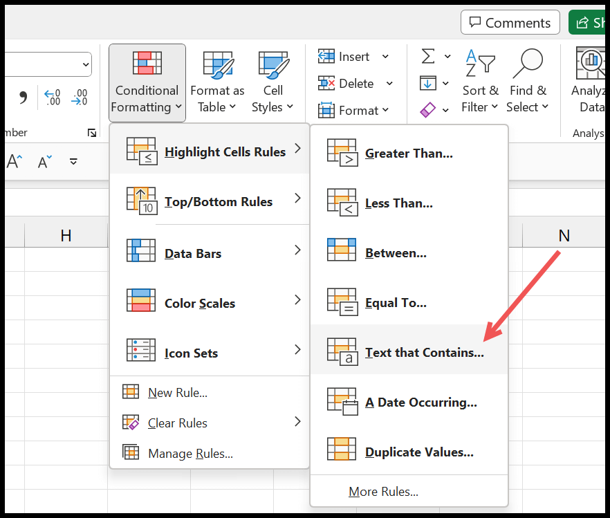
- Afterward, go to the Home Tab > Conditional Formatting > Highlight Cells Rules > Text that Contains.
- Next, in the dialog box, enter the text you want to look for in the data and select the formatting you want to apply to the matched cells.
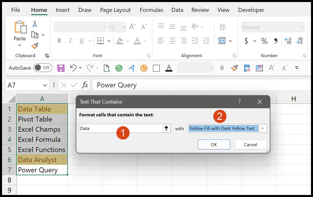
- In the end, click OK to apply the conditional formatting.
When you click OK, it will highlight all the cells where the text “Data” appears.
This option finds the text anywhere in the cell, and it’s not case-sensitive, so “data”, “Data” and “DATA” are all highlighted.
Highlight Cells That Contain Text using Custom Formula
The same formatting can be done with the help of a custom formula, and there is one plus point about this method: it applies conditional formatting based on another cell. That makes it dynamic; you don’t need to open the conditional formatting option to change the text.
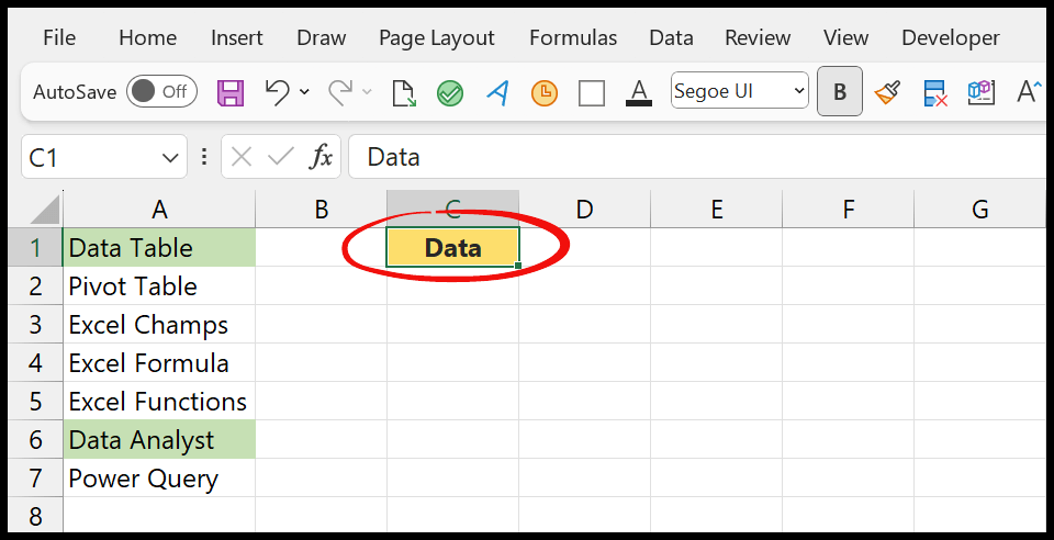
- Select the Data and go to the Home Tab > Conditional Formatting > New Rule.
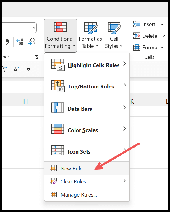
- In the new rule dialog box, click on “Use a formula to determine which cells to format”, and enter this formula in the formula input bar =AND($C$1<>””,SEARCH($C$1,A1)>0)
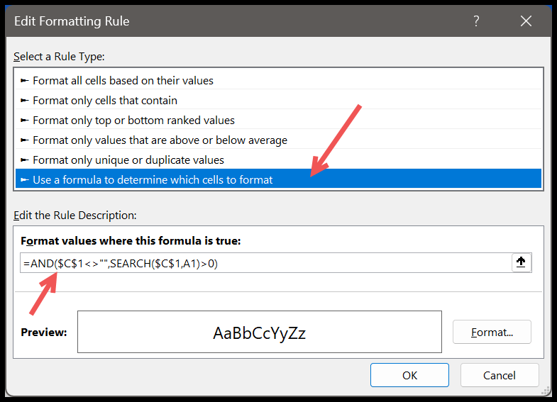
- Next, click “Format…” to specify the format you want to apply to the matched cells.
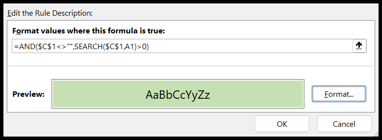
- In the end, click OK in the dialog box, and again OK to apply the formatting.
When you change the text in cell C1, the conditional formatting in the data will change.
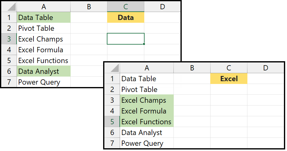
The formula that we have used tests two conditions:
- If Cell C1 is blank or not.
- Is the specified text in the data or not?
Let’s break down the formula to understand it.
- $C$1<>”” – It checks if cell C1 is not empty. If C1 contains any text or number, this part returns TRUE.
- SEARCH($C$1, A1) – Searches for the content of C1 within cell A1. If the content of C1 is found in A1, SEARCH returns the position of the first character.
- SEARCH($C$1, A1)>0 – Checks if the SEARCH function found the content of C1 in A1. If found, it returns TRUE; otherwise, SEARCH returns the #VALUE! error, and conditional formatting treats an error as FALSE, so the cell isn’t highlighted.
- AND($C$1<>””, SEARCH($C$1, A1)>0) – Combines the two conditions using AND. It returns TRUE only if both C1 is not empty and the content of C1 is found in A1.
The same rule with ISNUMBER returns a clean TRUE or FALSE instead of an error, which is easier to test in a cell:
=AND($C$1<>"",ISNUMBER(SEARCH($C$1,A1)))
Or you can also use the formula =COUNTIF(A1, “Excel”) > 0 in the conditional formatting to highlight cells that are exactly “Excel”. To match the text anywhere in the cell, add asterisks around it:
=COUNTIF(A1,"*Excel*")>0
If you just want to check if a cell contains text, you can use the ISTEXT function. This function tests whether a cell has text (and not a number) and returns TRUE or FALSE, according to the value in the cell.
Use a VBA Code to Highlight Cells with a TEXT
Below is a VBA code that refers to the range you have selected. When you run the code, it asks you for the text you want to highlight. Then, it highlights all the cells in the selected area where that text is with a yellow color.
Sub HighlightCellsContainingText()
    Dim searchText As String
    Dim rng As Range
    Dim firstCell As String
    Dim formatCondition As formatCondition

    ' Get the text from the user
    searchText = InputBox("Enter the text to highlight cells containing this text:", "Highlight Text")

    ' Exit if the user cancels the input box
    If searchText = "" Then Exit Sub

    ' Apply conditional formatting to the selected range
    Set rng = Selection
    firstCell = rng.Cells(1, 1).Address(RowAbsolute:=False, ColumnAbsolute:=False)

    ' Clear any existing conditional formatting in the selected range
    rng.FormatConditions.Delete

    ' Add new conditional formatting rule
    Set formatCondition = rng.FormatConditions.Add(Type:=xlExpression, Formula1:="=ISNUMBER(SEARCH(""" & searchText & """," & firstCell & "))")

    ' Set the formatting options (e.g., fill color)
    With formatCondition.Interior
        .Color = RGB(255, 255, 0) ' Yellow fill color
    End With
End Sub
To use this code, you need to open the Visual Basic Editor, insert a new module, and paste the code into the code window.
Note that the code first deletes any conditional formatting that’s already in the selected range, so select only the cells you want to apply the new rule to.
Case-Sensitive Match
Both the Text that Contains option and SEARCH ignore upper and lower case. If you want to highlight only the cells with the exact case, use FIND instead of SEARCH in the custom formula:
=ISNUMBER(FIND("Priority",A1))
Highlight the Entire Row or Multiple Words
To highlight the whole row when column A has the text, select the full data range (like A1:D20) and lock the column with a dollar sign in the formula:
=ISNUMBER(SEARCH("priority",$A1))
And to highlight a cell that contains any one of several words, put the words in an array inside SEARCH:
=SUMPRODUCT(--ISNUMBER(SEARCH({"priority","urgent"},A1)))>0
Frequently Asked Questions
Why is my rule highlighting the wrong cells?
The cell reference in the formula must point to the first cell of the range you selected. If you selected A2:A20, the formula should use A2, not A1; otherwise, each cell is checked against the cell above it.
Can I use wildcards in Text that Contains?
You don’t need them, as the option already looks for the text anywhere in the cell. In a COUNTIF formula, you do need the asterisks, like “*Excel*”.
Does it work with numbers?
Yes. SEARCH looks at the number as text, so searching for “25” highlights 125 and 250. For an exact number, use Highlight Cells Rules ➜ Equal To instead.

Written by
Puneet Gogia
Microsoft MVP — Excel · Founder, Excel Champs
Twelve years of teaching Excel, and a decade before that using it as a data analyst. Every tutorial here is written from a file I actually built.