

To average a range of times, use =AVERAGE(A1:A3) and make sure the result cell is formatted as time — Excel normally applies that itself. Times are stored as fractions of a day underneath, so averaging them works like averaging any other number.
Two things go wrong. If the result comes back as #DIV/0!, the times are stored as text rather than real times: they’ll be left-aligned in the cell, and the fix is =AVERAGE(TIMEVALUE(A1:A3)) entered with Ctrl+Shift+Enter on Excel 2019 or earlier, or converted properly with Data → Text to Columns → Finish.
And if you’re averaging durations rather than clock times — say task lengths that add up past 24 hours — format the result cell as [h]:mm with square brackets, or anything over a day gets truncated and you’ll see 3:15 where you should see 27:15.
For an average that ignores blanks or zeros, =AVERAGEIF(A1:A10,">0") works the same way here as with any number.

In this tutorial, we will learn to calculate the average of the time values you have in a range of cells.
Formula to Average Time
In the following example, you have three time values in column A in the range A1:A3. Now, you need to calculate the average of these time values.

For this, you need to use the AVERAGE function.
- First, enter the equal sign in a cell.
- Then enter the AVERAGE function and an opening parenthesis.
- Refer to the range where you have the time.
- In the end, enter the closing parenthesis and hit Enter to get the result.
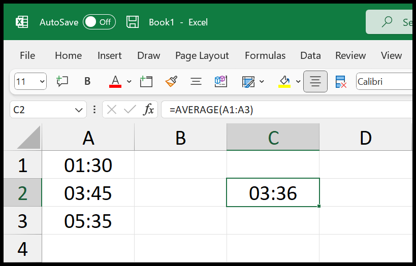
=AVERAGE(A1:A3)
In the cell where you want to calculate the average of the time, you need to make sure to have the time format on that cell. Even if you don’t change the format, Excel is smart enough to change this format for you when you enter the formula in it.
Understand Time in Excel
In Excel, when you enter time in a cell, Excel formats it automatically. There are two ways to format a time value: a 12-hour format and a 24-hour format. When you are averaging time and have a 12-hour format, you need to be a little cautious.
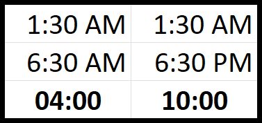
Above we have two different times: one is 6:30 AM, and the second is 6:30 PM. They look almost the same in the 12-hour format, but they are 12 hours apart, and that’s why the average is different with both formulas. So check AM and PM before you trust the result.
Why I’m Getting #DIV/0! Error While Averaging Time
If your time values are stored as a text value in the cell, you might face #DIV/0! error. Below we have a list of time values that are saved as text and on averaging we are getting an error.

To solve this problem, you can use the following formula, which converts the text to time values with TIMEVALUE before averaging (the range in your sheet may differ from the screenshot):
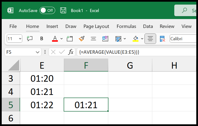
You need to enter this formula as an array formula by using Ctrl + Shift + Enter.
=AVERAGE(TIMEVALUE(A1:A3))
In Microsoft 365 and Excel 2021, you can just press Enter, as these versions handle arrays on their own.
Average Time with a Condition
To average only the times that meet a condition, use AVERAGEIF. The following formula averages the times in A1:A3 only for the rows where column E has “Mon”:
=AVERAGEIF(E1:E3,"Mon",A1:A3)
Round the Average Time to the Nearest Minute
The average often has seconds in it, like 10:11:40. To round it to the nearest minute, use MROUND with one minute as the multiple:
=MROUND(AVERAGE(A1:A3),"0:01")
And if you want the result as text with AM/PM, use TEXT:
=TEXT(AVERAGE(A1:A3),"h:mm AM/PM")
Average Times That Cross Midnight
If you average 11:00 PM and 1:00 AM, AVERAGE returns 12:00 PM (noon), because 1:00 AM is the smallest time value of the day. For times like bedtimes or night shifts, add one day to the times before noon, average them, and then take only the time part with MOD (press Ctrl + Shift + Enter in Excel 2019 and older):
=MOD(AVERAGE(IF(A1:A3<0.5,A1:A3+1,A1:A3)),1)
For 11:00 PM and 1:00 AM, this returns 12:00 AM (midnight).
Average Durations of More Than 24 Hours
If you are averaging durations (like hours worked) and the result can go over 24 hours, the normal time format starts again from 0. Format the result cell with the custom format [h]:mm to see the total hours.
Frequently Asked Questions
Why does my average time show a decimal number?
Excel stores time as a fraction of a day (12:00 PM is 0.5). Format the cell as Time, or with a custom format like h:mm, to see it as a time.
Does AVERAGE ignore blank cells when averaging time?
Yes. Blank cells are skipped. But a cell with 0:00 counts as midnight (0), so it pulls the average down.
How do I get the average time in minutes?
Multiply the average by 1440 (the number of minutes in a day) and format the cell as a number:
=AVERAGE(A1:A3)*1440
Written by
Puneet Gogia
Microsoft MVP — Excel · Founder, Excel Champs
Twelve years of teaching Excel, and a decade before that using it as a data analyst. Every tutorial here is written from a file I actually built.