

To sum only the rows a filter has left visible, use =SUBTOTAL(9,A2:A1001). A plain SUM adds everything in the range whether it’s filtered out or not, which is why your total doesn’t move when you filter. The first argument picks the calculation: 9 is SUM, 1 is AVERAGE, 2 is COUNT, 3 is COUNTA.
Use 109 instead of 9 if you also want to exclude rows you’ve hidden manually by right-clicking → Hide — for filtered rows the two behave identically, since SUBTOTAL always ignores those.
AGGREGATE does the same job with more control: =AGGREGATE(9,5,A2:A13), where 9 is SUM and 5 tells it to ignore hidden rows; option 7 ignores hidden rows and errors, which SUBTOTAL can’t do. To sum visible rows that also meet a condition, you need SUMPRODUCT with OFFSET, since SUMIF ignores filters entirely.
One shortcut worth knowing: Alt+= on a filtered range inserts SUBTOTAL automatically rather than SUM, and an Excel Table’s Total Row does the same.
Let’s say you have a list of weekly sales figures for different products in Excel. You’ve applied a filter to show only the sales for a specific product.
To find the total sales of this product, you would use a formula that can sum up only the visible cells showing the filtered results.
In Excel, to sum values only from the visible cells (that means when you have applied a filter), you need to use the SUBTOTAL function.
With this function, you can refer to the entire range, but the moment you apply a filter, it works dynamically and show the sum only for the visible cells.

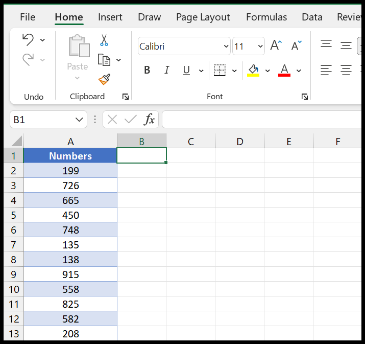
But apart from this there are also more formulas and function which you can use and today will explore all those. In the above example, we have a list of values in the column, and I want to create a formula that can show me the sum whenever I apply a filter to the column.
[thrive_leads id=’112075′]Use SUBTOTAL to Sum Only Visible Cells
SUBTOTAL helps you quickly calculate totals like sums, averages, or counts, but only for visible rows after applying a filter. It’s useful when you want to ignore any hidden rows in your data.
You choose what kind of calculation you want (like sum or count) and specify a range to check for visible cells. Follow the steps below:
- First, in cell B1 enter the SUBTOTAL function.
- After that, in the first argument, enter 9, or 109.
- Next, in the second argument, specify the range in column A, where you have the number.
- In the end, enter the closing parentheses and hit enter.

In the following snapshot, I have not yet applied the filter and it shows the sum of all the values that I have in the range.

Now to test this function you can add a filter and apply it. So, I’ll select 1,2, and 3 in the filter.

And the moment I hit enter it, shows the sum only for the filtered cells (visible).

Now, this function is dynamic and the moment you change the filter it changes the result value according to the visible cells.
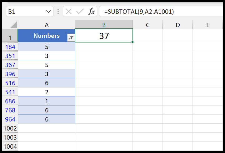
=SUBTOTAL(9,A2:A1001)
Using the AGGREGATE to Filter Visible Cells
AGGREGATE is a super function for calculating things like sums or averages. It can ignore hidden rows, errors, and even other subtotal calculations you’ve made, giving you clean results. You can pick the calculation type and tell it which cells to work with and what to ignore.
To count only the visible cells, you can use the below formula:
=AGGREGATE(9, 5, A2:A13)
This formula sums values from the range A2:A13. The ‘9’ tells Excel that you want to sum the numbers. The ‘5’ means Excel will ignore hidden rows.
The difference of AGGREGATE from SSUBTOTAL is that, it also ignores the hidden rows which has been hide manually.
Sum Visible Cells with a Criteria
To sum visible cells based on specific criteria in Excel, you can use an array formula that combines the multiple functions like SUMPRODUCT, SUBTOTAL, ROW, MIN, and OFFSET.
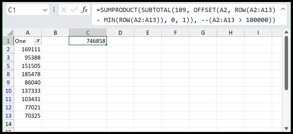
=SUMPRODUCT(SUBTOTAL(109, OFFSET(A2, ROW(A2:A13) - MIN(ROW(A2:A13)), 0, 1)), --(A2:A13 > 100000))
This formula helps you add values from A2 to A13, but only in two cases: the cells must be visible (not hidden by a filter), and each cell’s value must be greater than 100,000.
- SUBTOTAL(109, OFFSET(…)) – This part checks each cell from A2 to A13 to see if it’s visible or not.
- OFFSET(…) – Go to each cell in the range, one by one.
- ROW(A2:A13) – MIN(ROW(A2:A13)) – This calculates the position of each cell in the range to ensure the OFFSET works correctly.
- –(A2:A13 > 100000) – This checks if the cell’s value is more than 100,000, then turns the true/false result into 1 or 0.
- SUMPRODUCT(…) – This multiplies the visible and qualifying (more than 100,000) cell values together and sums them up.
Written by
Puneet Gogia
Microsoft MVP — Excel · Founder, Excel Champs
Twelve years of teaching Excel, and a decade before that using it as a data analyst. Every tutorial here is written from a file I actually built.