Using VLOOKUP in a VBA Code

This tutorial will teach us to use VLOOKUP in a VBA code. Make sure to read the entire article, or you can also watch the video tutorial.

How to use VLOOKUP in VBA?

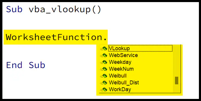
If you want to use VLOOKUP in VBA, you need to use the WORKSHEETFUNCTION property, which allows you to access all the functions. When you insert WorksheetFunction, you can get the list of the functions to choose VLOOKUP from there.

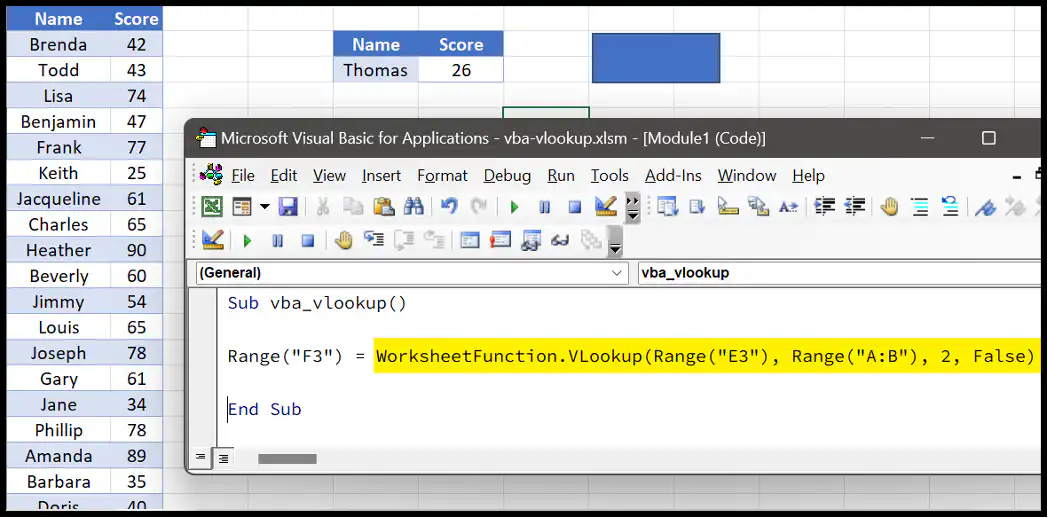
In this example, we have a list of students where we have the name and the score. We need to write a code with VLOOKUP to get the student’s score by using the name as a lookup value.

Steps to Write a VBA Code to use VLOOKUP in Excel

1. First, enter the WorksheetFunction property and press the (.) dot to get the function list.
2. Next, enter VLOOKUP or select it from the list.
3. Now, enter the starting parentheses to start the function.
4. After that, specify the arguments of the VLOOKUP function. (Ahead in this post, I have shared detailed steps to specify the arguments)
5. In the end, specify a range of cells to get the result of the function.

Range("F3") = WorksheetFunction.VLookup(Range("E3"), Range("A:B"), 2, False)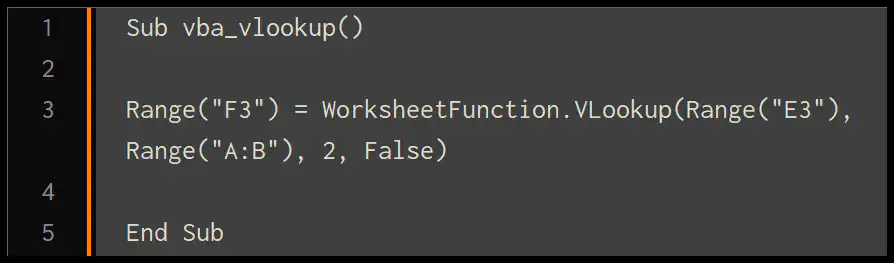

Define Arguments in the VLOOKUP in VBA

Using a worksheet function in a VBA code using the worksheet function property won’t show you the names of the arguments you need to define.

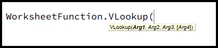
So that’s why you need to know the arguments you must specify in the function.

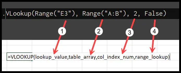
In VLOOKUP, there are four arguments to define:

1. In the first argument, you need to define the value which you want to look for in the data. In our example, we need to define the cell with the value, so we have used a range object to specify the cell E3.
2. In the second argument, you need to define the table (data) from which you want to look for the value. And we have again used a range object to specify range A:B.
3. In the third argument, we need to define the column index number, which tells the function of the column number from which we need to get the result value. In our example, we have specified 2.
4. In the fourth argument, we need to define the match type (exact or appropriate). As we need to do an exact match, we have used FALSE.

Once you specify all the arguments, you need to get the result of the function in a cell or through a message box. That’s why, in the code, we specified the cell F3 to get the value.

Using VLOOKUP in VBA for Multiple Values

If you want to apply VLOOKUP to get results for multiple values, you can use a code like the following.

Sub vba_vlookup()
Dim i As Integer
Dim lookup_start As Range
Set lookup_start = Range("E2")
i = 5
For i = 1 To i
    lookup_start.Offset(i, 0) = WorksheetFunction.VLookup(lookup_start.Offset(i, -1), Range("A:B"), 2, False)
Next i
End Sub

In the above code, we have used the FOR NEXT LOOP to loop the VLOOKUP for five cells down words. 

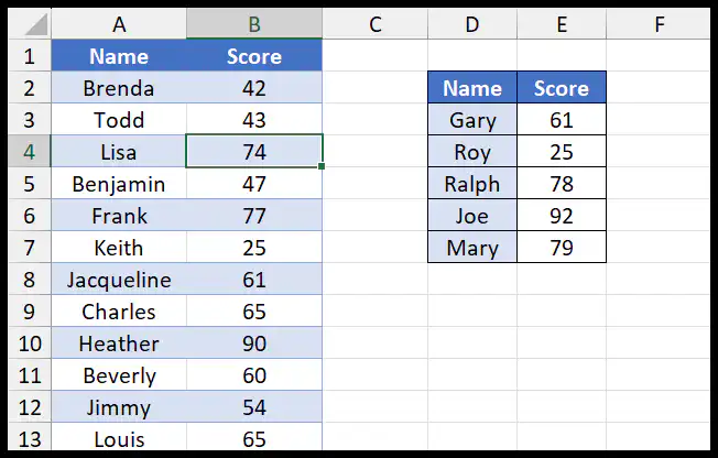
In our data, we have five values for which you need to lookup for the score. These values are in the range D3:D7, and we need to get the score in the range E4:E7.

This code starts from the cell E2, uses offset to go to the cell from E3 to E7, and uses VLOOKUP to get the score for your values in the corresponding cell (Column D). As we have five values for the lookup, we have used 5 in the look counter.