How to Apply Strikethrough in Google Sheets

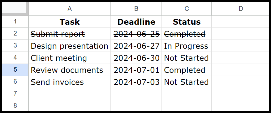
Let’s say you’re managing a project and keeping track of tasks in Google Sheets. You have a list of tasks in one column, and as you complete each task, you want to mark it clearly without deleting it. To do this, you can use the strikethrough.

There are five ways you can use in Google Sheets to apply strikethrough.

1. Use the keyboard shortcut Alt + Shift + 5 to apply the strikethrough.
2. Go to Format > Text > Strikethrough.
3. Click the strikethrough button on the toolbar.
4. Use a Google App Script to apply strikethrough.
5. Use a checkbox to apply strikethrough.

In this tutorial, we will learn all these four methods in detail.

Keyboard Shortcut to Apply Strikethrough

To quickly apply strikethrough in Google Sheets using a keyboard shortcut, select the cell or the text within the cell that you want to strikethrough.

• Press Alt + Shift + 5 if you’re using Windows.
• Press Command + Shift + X if you’re using a Mac.

This will immediately add a line through the values in the selected cells, indicating that the task or item has been completed.

If you want to apply strikethrough partially to a value in the cell, edit the cell and then use any of these keyboard shortcuts.

Apply Strikethrough from the Format Menu

You will get the strikethrough option if you go to the format menu. You can use the below steps to use this option.

1. First, select the cell or the range within the cell that you want to strikethrough.
   
2. Now, go to the top of the screen and click on the “Format” menu.
3. Then, from the dropdown menu, hover over “Text”.
4. In the end, click on “Strikethrough” in the submenu that appears.
   

This will add a line through text in the selected cell of the range of cells, marking it as completed.

Apply the Strikethrough Button from the Toolbar Button

To use the strikethrough button from the toolbar, select the cell or the text within the cell you want to strikethrough.

Go to the toolbar at the top and look for the strikethrough button (which looks like the letter “S” with a line through it).

This will instantly apply the strikethrough formatting to your selected cell or the range.

Create a To-Do List with Checkboxes and Conditional Formatting

1. First, add tasks in a column, select the corresponding column, and then go to the Insert > Checkbox to insert the checkboxes into the selected cells.
   
2. Now, select the cells where you have, and you want to format with strikethrough based on the checkbox. Then, go to the menu and click on Format > Conditional formatting.
   
3. In the “Conditional format rules” sidebar, set the format rules as follows:

   • Format cells if: Choose Custom formula is.

   • Formula: Enter the formula =$F2=TRUE (adjust the cell reference $F2 to match the location of your checkbox).
   • Click on the Strikethrough button.
     
4. In the end, click Done to apply the conditional formatting. And now, whenever you checkmark a checkbox, it will strikethrough the task.