Key Points
- SUMIFS uses AND logic by default. It only sums rows where all conditions are true.
- To apply OR logic, use an array constant inside SUMIFS and wrap it in SUM.
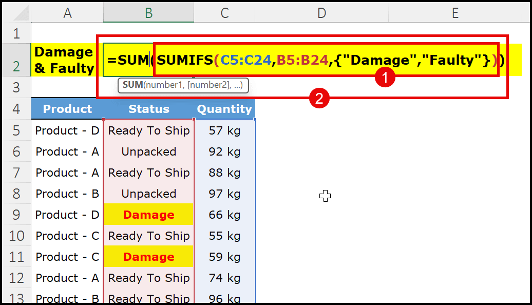
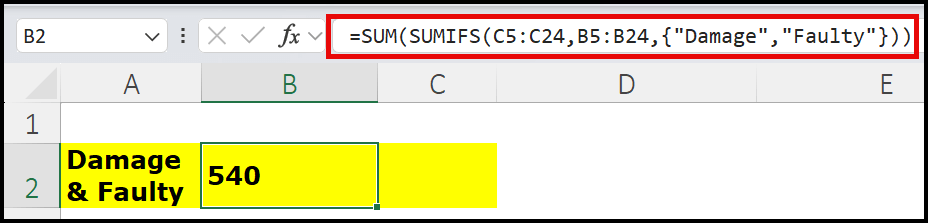
- Formula to use: =SUM(SUMIFS(C5:C24, B5:B24, {“Damage”,”Faulty”}))
- In Excel 365, formulas spill automatically; in older versions, you may need Ctrl+Shift+Enter.
- You can also keep your OR criteria in cells (like E2:E3) and reference them in SUMIFS.
- For AND + OR together, add an extra condition in SUMIFS or use SUMPRODUCT for more control.
- SUMPRODUCT allows both OR (+) and AND (*) in one formula, no CSE needed.
- If you need case-sensitive OR, use EXACT inside SUMPRODUCT.
In Excel, the SUMIFS function works with AND logic, which means you can specify more than one condition to sum values. When you apply multiple conditions, SUMIFS will only include those cells where all conditions are met together and then return the sum.
But, in real situations, you may sometimes want to add values using OR logic.
OR logic means you sum values where either one condition or another condition is met, and both conditions work independently. The limitation is that SUMIFS does not support OR logic by default, so you need alternative way to write a formula to achieve this.
Below is a generic formula to use or condition logic with SUMIFS:
=SUM(SUMIFS(Quantity, Status, {“Damage”,”Faulty”}))
Understanding OR Logic (Multiple Criteria)
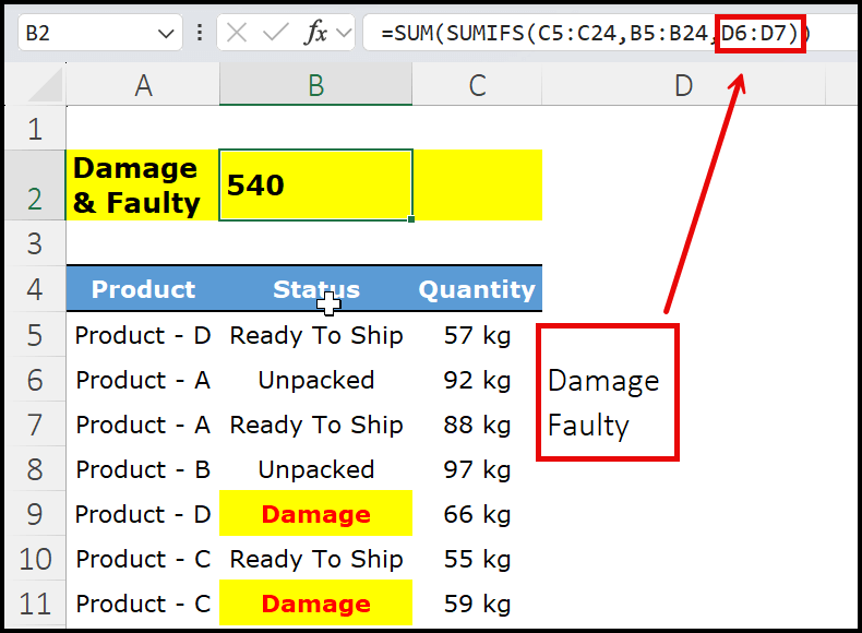
Let’s understand this with a real-life example. Suppose I have product data with three columns: Product, Status, and Quantity. In the Status column, I have different entries like Ready to Ship, Unpacked, Faulty, and Damaged.
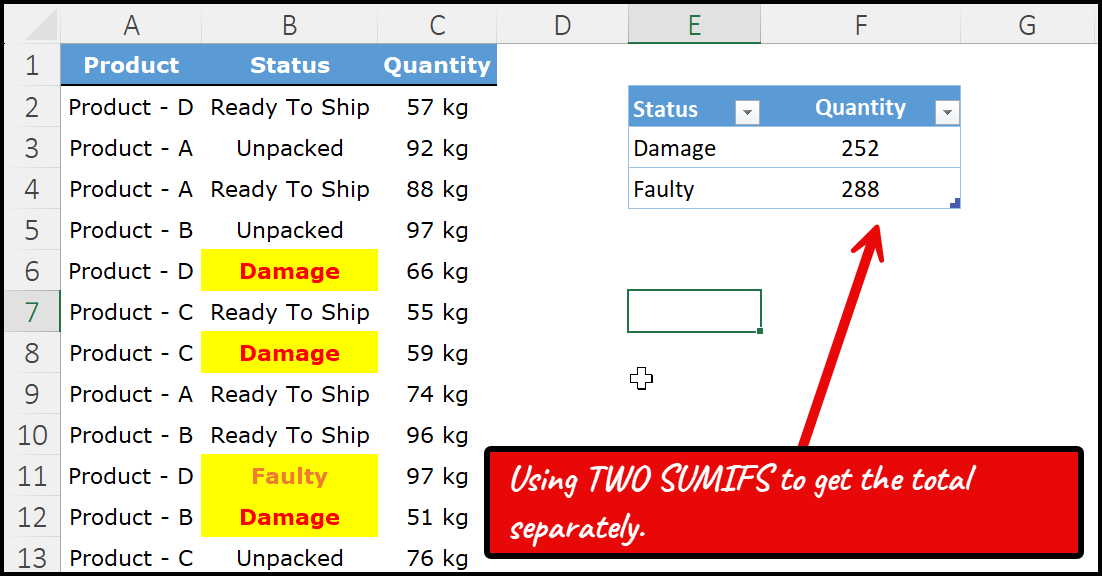
Now, if I use the SUMIFS function, it works with AND logic, so I can easily calculate the total quantity for one specific status, such as Damaged or Unpacked.
For instance, in the example above, when I use SUMIF to calculate the quantity for Damaged and Faulty separately, I get 252 for Damaged and 288 for Faulty.
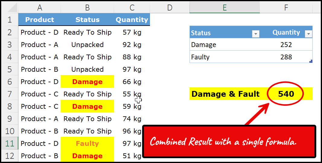
And when I apply an OR logic workaround with SUMIFS, instead of showing two separate results, I get the combined total in a single cell. The result is 540, which represents the total quantity of both Damaged and Faulty products together.
Quick Refresher on SUMIFS
I’m sure you’re already familiar with how the SUMIFS function works but let me give you a quick refresher. SUMIFS helps you sum values from a column or range based on multiple criteria. You can specify conditions across different columns, and Excel will only include the rows that meet all those conditions. From there, it returns the total from your main sum column.
=SUMIFS(sum_range, criteria_range1, criteria1, [criteria_range2], [criteria2], …)
Write the Formula to use OR Logic in SUMIFS
I’ll continue with the same example to help you understand how to write the SUMIF function with OR logic. First, let’s look at the sum_range argument. This is the column where Excel will sum up the values once the conditions are applied.
In our example, the Quantity column is in the range C2:C21, so that’s the sum range we’ll use in the formula.
After that, in the second argument, which is the criteria_range, you need to specify the column that contains the statuses. In our example, that would be the Status column.
Then, in the third argument, you enter your criteria. Now, here is where we need to make a small change. Normally, when you use SUMIF or SUMIFS, you specify a single condition at a time.

But in this case, we want to apply two conditions at once. To do that, we use curly brackets {}. You start by opening the curly bracket {, then type your first criteria, which is “Damage” (enclosed in double quotation marks because it’s text), followed by a comma.
Next, you type your second criteria, “Faulty”, again inside double quotation marks. Finally, close the curly bracket }. This way, Excel will understand that you want to include both statuses together in your calculation.
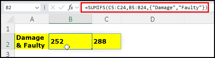
Now, here’s what happens when you write your SUMIFS formula this way and press Enter. You won’t get the combined total for both statuses immediately. Instead, if you are using Excel 365, the formula will return an array with two values, one showing the quantity for Damaged and the other showing the quantity for Faulty.
You might wonder, “Why are we writing this formula if it still gives two separate values?” The answer is simple, we just need one more step. To get the total quantity for both statuses in a single value, you simply wrap your SUMIFS formula inside the SUM function.
Once you do this and press Enter, Excel will add those two values together and return the combined total to one cell.
Apart from specifying both criteria directly inside the formula using curly brackets, there’s another way to do this. You can enter both conditions into two separate cells, placed next to each other in a continuous range.
After that, instead of writing the criteria directly in the formula, you simply refer to those cells in the criteria argument of your SUMIFS function.
This approach works the same way as writing the conditions inside curly brackets, but it has an added benefit. It makes your formula easier to update. If you ever need to change, you can just update the cell values instead of editing the formula.
Old Vs. New Excel Versions
If you are using an older version of Excel, you need to enter this type of formula with CTRL + SHIFT + ENTER instead of pressing Enter normally. This tells Excel to treat it as an array formula. If you are using Excel 365, where dynamic arrays are already supported, you don’t need to use this keyboard shortcut. You can simply enter the formula like any other, and Excel will handle it automatically. In Excel 365, formulas that return multiple results, like our SUMIF example when using curly brackets, will spill the results into the cells below or beside the formula cell.
How this Formula Works?
As I said, the SUMIFS function uses logic to sum values. But the formula which you have used above includes an OR logic in it. To understand this formula, you have to split it into three different parts.

The first thing is to understand that you have used two different criteria in this formula by using the array. Learn more about the array from here.
The second thing is when you specify two different values using an array, SUMIFS has to look for both values separately. The third thing is even after using an array formula, SUMIFS cannot return the sum of both values in a single cell. That’s why you have to enclose it with the SUM.
Using OR LOGIC & AND Logic at the Same Time
Think about a situation where we need OR logic in SUMIF, but we also need one more condition with it. Here’s the situation: we want to sum quantities for Damage or Faulty, and we also need to apply a condition for Product D. In other words, we want the quantity for Product D, but only for rows marked Damage or Faulty.
We’re still using OR for Damage/Faulty, but we’re narrowing it down further with an AND condition for Product D. For this, we should move from SUMIF to SUMIFS.
By now, you already know how to use the SUMIF function, and SUMIFS is basically an extended version of SUMIF that lets you specify multiple criteria to get the sum from a column. With SUMIFS, we’ll first add a criterion to test Product D, which narrows the data from all products to only Product D.
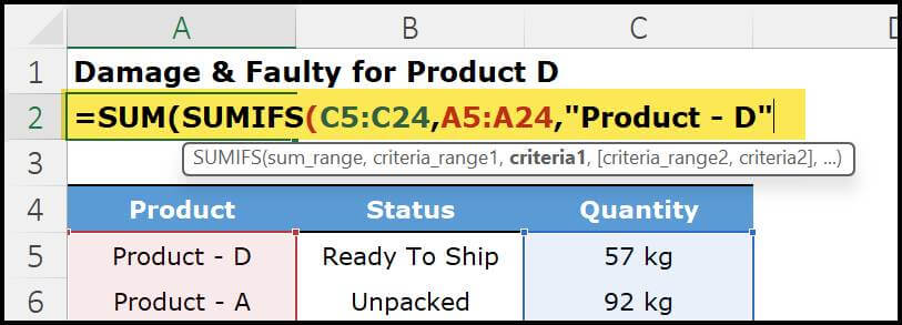
After that, we’ll add an OR condition in the second criterion to sum quantities for Damage or Faulty. So, first we filter to Product D, and then we apply OR logic for Damage and Faulty. Below is the formula we’re going to use.
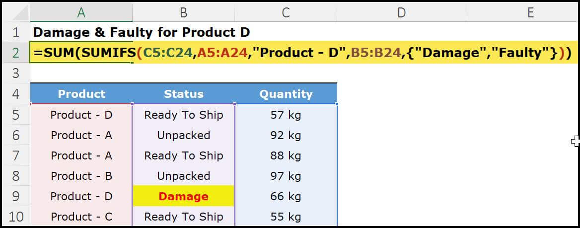
As you can see above, we wrapped the SUMIFS function inside SUM to add the results for both conditions, Damage and Faulty.
If you’re using an older version of Excel without dynamic arrays, enter the formula with CTRL+SHIFT+ENTER so Excel can take the array returned by SUMIFS when using OR logic. In Excel 365 or with dynamic arrays, just press Enter.
Using SUMPRODUCT to Create a the Same OR LOGIC to SUM VALUES
You can achieve the same result with SUMPRODUCT. The best part is that SUMPRODUCT lets you build the entire OR and AND logic in a single formula, and you don’t need to use CTRL+SHIFT+ENTER, even in non–dynamic array versions of Excel. Here’s the formula you can use to get the same result from the data.
=SUMPRODUCT(
   (A5:A24="Product - D") *
   (
      (B5:B24="Damage") +
      (B5:B24="Faulty")
   ) *
   C5:C24
)
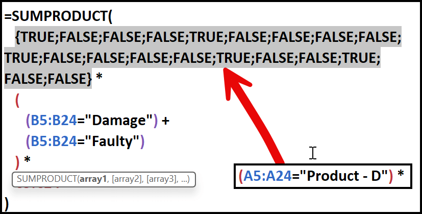
In the first part, we have a single condition to test: Product D. We reference column A (where product names are) and set the criterion to “Product D.”
Then we multiply this condition by the second part of the formula. In SUMPRODUCT, the asterisk performs logical AND, so a row is counted only if it meets both tests: Product D. This first filter narrows the data to Product D, and everything that follows applies only to this product data only (Product – D).
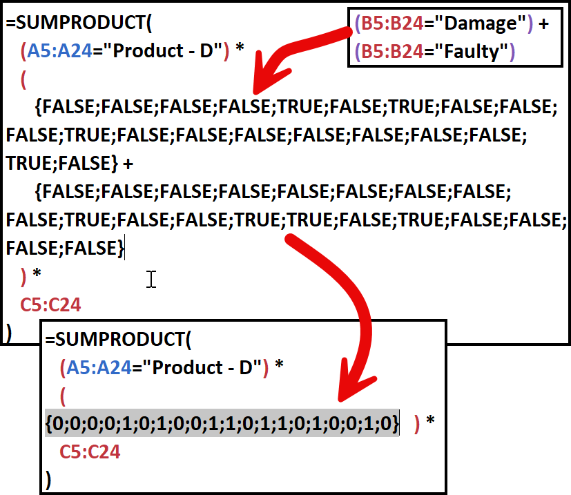
In the second part, we test the Status column twice, once for “Damage” and once for “Faulty”. And place a plus sign between those two conditions.
Each condition returns a TRUE/FALSE array; adding them with the plus sign applies OR logic. This addition effectively marks a row as TRUE if it is either Damage or Faulty. So, this second part is what gives us the OR logic for Damage and Faulty.
In this formula, we test three conditions arranged in two parts. First, we filter the data to Product D. Second, we apply OR logic on the Status to include Damage or Faulty.
Together, that gives us rows where Product = D and Status is either Damage or Faulty.
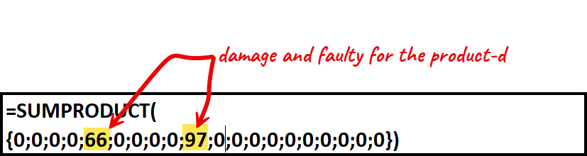
Next in the third, we bring in the Quantity by multiplying this logical array by the Quantity column (column C). Because SUMPRODUCT multiplies and then sums, this returns the total Quantity only for Product D with Damage or Faulty.
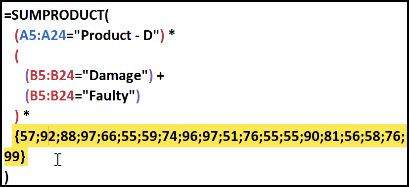
In the end, after combining all three arrays, we get a final array of quantities for Product D, but only from the rows where the Status is Damage or Faulty.
Case-sensitive OR Logic in SUMIF
When you use SUMIF or SUMIFS with OR logic, Excel performs a non–case-sensitive match. If you need an exact, case-sensitive match while summing with OR logic, switch to SUMPRODUCT.
Inside SUMPRODUCT, use the EXACT function to use case sensitivity so the calculation only includes entries that match the text exactly.
=SUMPRODUCT( (EXACT(B5:B24,"DAMAGE") + EXACT(B5:B24,"FAULTY")) * C5:C24 )
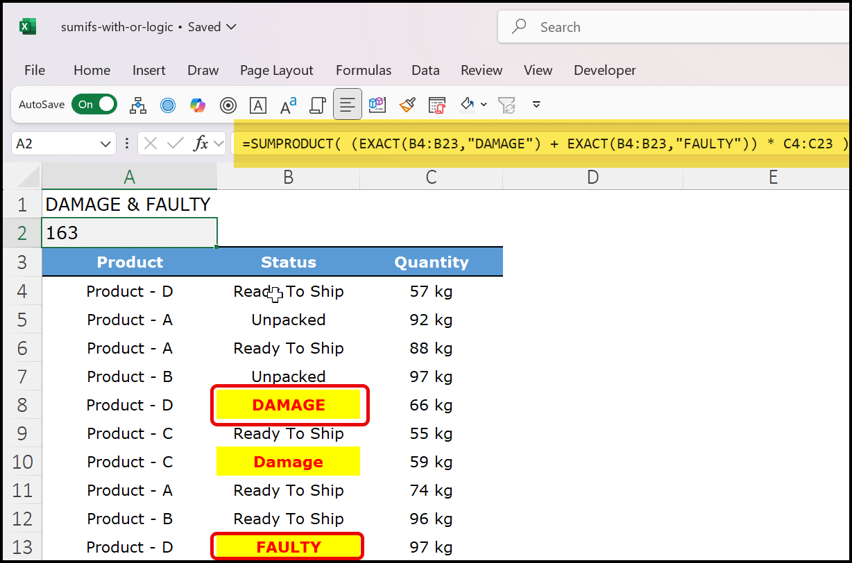
In the formula above, we use SUMPRODUCT together with EXACT to perform a case-sensitive OR logic sum. First, EXACT tests the Status column for the texts “DAMAGE” and “FAULTY”, both intentionally written in CAPITAL letters to enforce case sensitivity.
Each EXACT returns an array of TRUE/FALSE values; we add these two arrays to combine them into a single OR array that marks rows where the status is exactly “DAMAGE” or exactly “FAULTY” (both in CAPITAL case).
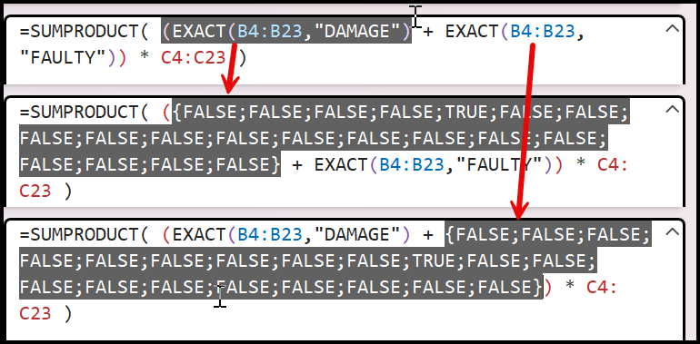
Next, this combined array is multiplied by the QUANTITY column, so only quantities from matching rows are kept.
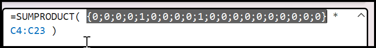
Finally, SUMPRODUCT adds those quantities, returning the total for rows where the status is DAMAGE or FAULTY in CAPITAL case.

Frequently Asked Questions (FAQ)
No, SUMIFS cannot handle OR logic on its own. It applies AND logic, meaning all conditions must be true at the same time. However, you can work around this limitation in two ways. The most common method is to provide an array of criteria inside curly brackets (e.g., {“Damage”,”Faulty”})
If you’re using Excel 365 or a version that supports dynamic arrays, you don’t need Ctrl+Shift+Enter. Just press Enter and Excel will handle the array automatically. In older versions of Excel, formulas that use array constants (like {“Damage”,”Faulty”}) may require Ctrl+Shift+Enter to calculate correctly.
Last Updated: 01-Oct-2025
I never leave a comment but holy cow that was really useful and easy to follow. Thanks for sharing.
hi i just to try out on this formula, which I still could not get it done, I am doing a bank recon, at the end of the month. there are some cheque are not clear which mean the other side of the party has not bank in the cheque. now this few cheque will carry forward to next month. how am i going to do this formula out? I need to tally with the bank amount in my exit excel worksheet.
what if I have “Damage” and ”Faulty” in the same field and I only want to sum it once?
Try using the symbol *, like this: =SUM(SUMIF(B2:B21,{“*Damage*”,”*Faulty*”},C2:C21))
Lovely article Puneet, but I have question in my mind, how if this criterias in bracket {“Damage”,”Faulty”} change to cell refference?
Thanks
A doubt, and if it is to sum everything that is different from “Demage”, “Faulty”?
Hi Puneet,
Many many thanks for the multiple criteria use within SUMIFS.
I was struggling with my formula being all in ‘one cell’ using different criteria but same criteria range. Your solution and brilliant explanation using the SUM function solved that in seconds!
Many thanks once again.
Keep up the good work!
You are welcome, Irene.
THE ABOVE MENTIONED INFO IS VERY USEFUL TO ME, THANKING YOU
Great! I really like to read ur posts. Excel formulas and usage facinates me a lot. I work with data so ur examples help me a lot… Thanks.
Hey champ, I need your help to resolve my query. I want to make the criteria dynamic by getting the input from the user using slicer. When I have multiple criteria for same column I can use sum before sumifs as hard coded formula but I want to get the criteria from slicer based on the selection by the user. How to do this?
One word – amazing.
thanks!
Thanks for your word…
Building on the formula above =SUM(SUMIFS(D2:D21,B2:B21,{“Damage”,”Faulty”},C2:C21,”No”))….
Why can you not reference cells instead of using “Text”?
=SUM(SUMIFS(D2:D21,B2:B21,{B$6$,B$11$},C2:C21,C$11$))
Apologies, I re-read the article and saw the named range +CSE.
Very useful article. Thanks
What does “named_range” mean? What do you input as “named_range” when doing a cell reference instead of written words? So confused :/ Do you put the cell range of the values you want to look up?
Hi
I am trying to use this formula and its not adding correctly
=SUM(SUMIFS(D2:D21,B2:B21,{“Damage”,”Faulty”},C2:C21,”No”))
any clue what might I have done wrong ?
Hi Puneet,
Your tips above are highly effective, and I have a secondary challenge to apply here! Hope this post isn’t too old to be reignited 🙂
I may simply be thinking about this before having coffee every time but I can’t seem to solve it conceptually.
Effectively I’m looking for a way to dynamically ADD or REMOVE criteria from a SUMIFS without using multiple sums under IF conditions.
Example:
Name | Gender | Category | Sales
———————————————-
Dave | Male | A | 20
Mike | Male | B | 30
Tracy | Female | C | 10
Sam | Female | D | 80
I have many more categories in my working problem, including date ranges etc (effectively invoice data summarised).
I’m using a SUMIFS and I’d like to dynamically pick Male, Female or BOTH.
For both my assumption is that I should dynamically remove the criteria on Gender to include BOTH.
My only requirement is to do this in a single formula/array without an IF condition as mentioned.
Thoughts?
Cheers
Dave
Hi – What if I wanted to look at Damaged OR Faulty, and control for products, like only Product B and Product C. Can you have two OR sections?
Range_Name Critaria is Awesome and Very Helpful
Great Work Puneet
From Rizwan Planning Engineer
I’m glad you linked it.
Oh wonderful. I’m still mastering it inorder to know how to use it offhand.
That’s great. Keep it up.
Thanks for a great tip! Is it possible to use a dynamic criteria inside the OR Logic? i.e. use cell referance instead of {“Damage”,”Faulty”}?
Hey Shay, thank you very much for hitting me back. Your question is super awesome. So, if you want to create a dynamic reference, first you need to refer to a named range (the best way is to use a table reference) instead of adding your values in curly brackets. Secondly, you have to enter the formula with CSE as a proper array formula and, it works like a magic. Tell me if you need any further help.
Works Like a charm. thanks again for the quick and proffesional reply
Yo. ../
Hi shay,
Can u please help me to use dynamic criteria ??
Nice that is working without CSE. Just wondering if calculation time is faster then doing 2 seperate SUMIFs/SUMIFSs and then adding up. For larger datasets that can be an issue.
Yes, it is faster than using two different calculations. But, will effect you once you try to add more criteria.
Very useful tip, Puneet. Thanks for sharing.
I’m so glad you liked it.
Hi Puneet,
Formula is awesome. sum up using OR logic in sumifs for multiple criteria where its matching. i sum up multiple criteria where its matching but i need sum up where criteria doesn’t match under others head. can you please help me on this.