The UNIQUE function in Excel extracts unique values from a list. It identifies unique entries and removes duplicates, providing a distinct list of values. This function is helpful for data analysis, simplifies lists, and ensures data accuracy by eliminating repeated values.
You can also use UNIQUE to get unique rows from a table, combine them with other functions, count unique values, create a named range of unique values, and do much more.
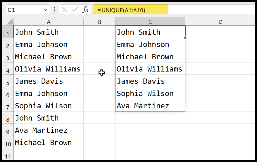
To understand it quickly, you can check out the example below, where we have names in the A1:A10 range. The formula =UNIQUE(A1:A10) extracts the unique names from the range and removes any duplicates.
In this tutorial, we will learn about Excel’s UNIQUE Function in detail and explore some examples to understand how to use it in the real world.
Syntax of UNIQUE Function
Now it’s time to understand the syntax of the unique function so that you can use it with its full power…
=UNIQUE(array, [by_col], [exactly_once])
In this syntax, you have three arguments to define. Out of these three arguments, two arguments are optional.
- array – This refers to a range of cells or an array where you have values and want to get only unique values.
- [by_col] – This argument is optional. You can specify it as TRUE or FALSE. When you specify TRUE, it tells the function to compare values by column, and FALSE tells the function to compare values by column.
- [exactly_once] – This argument works in two ways. With TRUE, it returns only the values that appear exactly once in the array. With FALSE, duplicate values are removed, and the unique list is returned.
Get Unique Values with UNIQUE Function
Let’s start with the example we have seen before this tutorial. From the list of names, we have a list of names. To write a formula for this, you can use the below:
- Enter the UNIQUE Function.
- In the first argument (array), refer to the range A1:A10.
- In the second argument (by_col), specify FALSE only to get the unique rows as we only have one column.
- In the third argument (exactly_once), specify FALSE to return every distinct item.
- At last, hit enter to get the result.
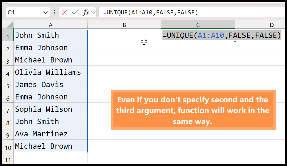
=UNIQUE(A1:A10,FALSE,FALSE)
Note: The function will work similarly even if you don’t specify the second and third arguments.
When you hit enter to get the result, it returns a new array with all the distinct values. In the example below, the result array has seven distinct names in the C1:C7 range.
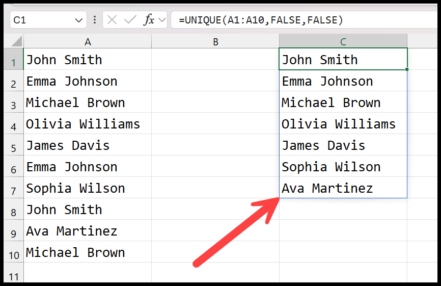
As you can see in the above screenshot,
Get values that appear only once
The UNIQUE third argument allows you to get values in two ways. The first is what we have seen in the above example. However, you can also get the values that appear only once on the list.
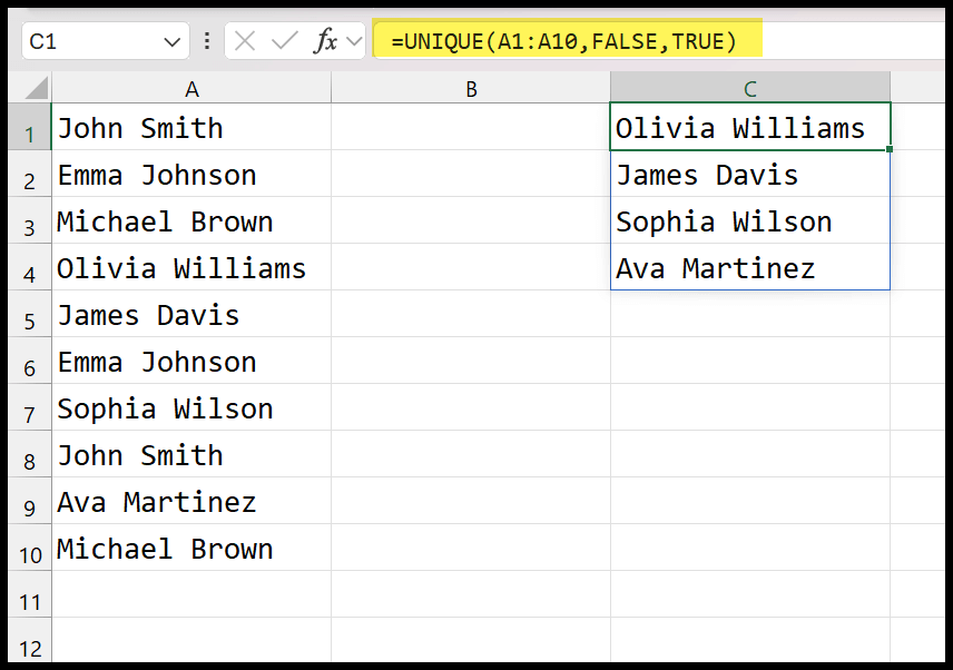
=UNIQUE(A1:A10,FALSE,TRUE)
The above formula helps you get the list of names that appear only once in the range A1:A10. The first argument, A1:A10, tells Excel where to look for the names. The second argument (by_col), FALSE, tells Excel to focus on rows, which is useful when dealing with one column of data.
Count Unique Values using UNIQUE and COUNTA.
Now, let’s take the same example, but instead of getting unique names, count the number of unique names. To do this, you need to combine the COUNTA with UNIQUE.
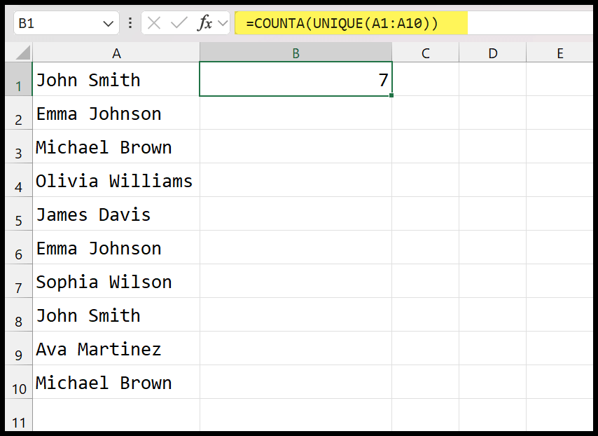
The UNIQUE part of the formula extracts the unique names from the range A1:A10. As you can see, the range has ten names, and UNIQUE removes the duplicates and returns only the distinct names.
After that, COUNTA counts the values from the array/list returned by UNIQUE. The range A1:A10 has 7 unique names, so the result in cell B1 is 7.