

Open Home → Conditional Formatting → Manage Rules, set Show formatting rules for to This Worksheet, and compare each rule’s formula with its Applies to range. Most broken rules point at the wrong cell: a rule on A2:A12 must be written for A2, as in =A2>1200, not A1.
Check the dollar signs next. =$A$2>1200 tests the same cell for every cell in the range, so everything or nothing is highlighted. Use =A2>1200 to test each cell on its own, or =$A2>1200 to colour whole rows from one column.
If every cell lights up, the numbers are probably stored as text: Excel ranks any text above any number, so A2>1200 is TRUE for all of them. Convert them with the warning triangle’s Convert to Number or Data → Text to Columns → Finish, or test =VALUE(TRIM(A2))>1200 when stray spaces are the cause.
When two rules clash, the one higher in Manage Rules wins, so a yellow “over 500” rule placed above a green “over 1000” rule turns the over-1000 cells yellow too. Move the stricter rule up, or tick Stop If True on it. A formula that returns a number still counts: any non-zero result is treated as TRUE, so =A2+100 formats nearly every cell.
Excel does not accept structured references such as Table1[Sales] in a rule, so use normal references such as $C2. A function your version lacks, such as TEXTJOIN before Excel 2019, returns #NAME? inside the rule and nothing is formatted. On a protected sheet existing rules keep working, but you cannot add or edit rules until you choose Review → Unprotect Sheet.
You have a sales report in Excel and want to highlight cells with sales over $1000 using conditional formatting. You set up the rule, but nothing changes in your cells.
One common reason is that your sales data has extra spaces or text, making Excel read the values as text instead of numbers.
In Excel, when you use conditional formatting, sometimes you apply it, but it doesn’t work. In this situation, you need to troubleshoot the formatting you have used.
While applying pre-defined conditional formatting, you might not face issues, but when using custom formulas, there’s a good chance you will.
1. Incorrect Reference
When you apply conditional formatting using the formula, you may refer to a different cell by mistake. See the example below: The range where I want to apply the conditional formatting rule is A2:A12.

And the formula needs to refer to cell A2 instead of A1. And because I referred to A1 in the formula, the rule has been wrongly applied.
You can see that the condition is to test if the value is greater than 1200 or not, and it has highlighted cells even when the value is not greater than 1200. It is all because of the wrong reference.
When working with conditional formatting, one of the major reasons for it not working is the wrong reference. The formula must refer to the first cell of the range in “Applies to” (here, A2).
2. The Result of the Condition Needs to be TRUE or FALSE
In conditional formatting, the result of the condition must be TRUE or FALSE. If your formula doesn’t return TRUE or FALSE, the rule won’t work the way you expect. When a formula returns a number, Excel treats any number other than 0 as TRUE, so the rule highlights almost every cell; and a formula that returns text or an error never applies the format.
To fix this, write your formula to produce a TRUE or FALSE result. For instance, use a comparison operator like =A1>100 instead of =A1+100 (which returns a number and highlights nearly everything). This way, the formula checks if the condition is met (TRUE) or not (FALSE). Correcting your formula ensures Excel can apply the conditional formatting rule properly.
Enter the formula in a worksheet cell first to see what the result turns out to be.
3. While Copying and Pasting the Conditional Formatting
If you have an absolute reference in the formula and copy and paste the conditional formatting to a new cell or a range of cells, the format will apply with the wrong condition.
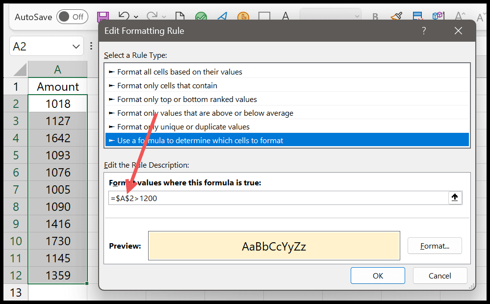
In the above example, our reference is absolute; you can see the dollar signs. And when you copy and paste this conditional formatting to a new place, it will always refer to cell A2. Remove the $ before the row number (or both $ signs) so that the reference moves with each cell.
4. When Numbers are Formatted as Text
Incorrect data format is a common reason why conditional formatting might not work. It happens when the data in your cells isn’t stored as the right type.
For example, numbers may be stored as text because of extra spaces, non-numeric characters, or being formatted as text. Excel can’t apply conditional formatting correctly if it doesn’t recognize the data type.
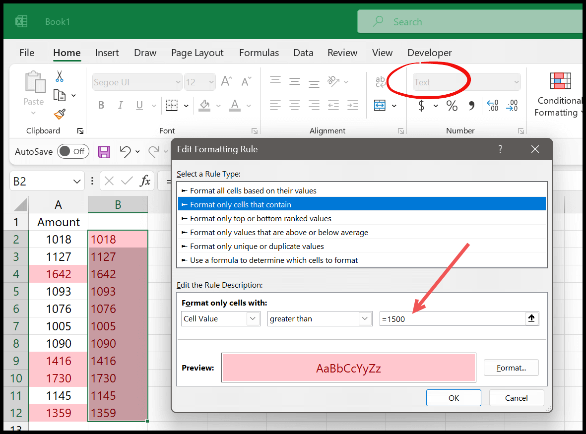
In the above example, columns A and B have the same conditional formatting rule, which tests the numbers above 1200. But in column B, the numbers are entered as text, and the rule highlights all of them. That’s because, when Excel compares text with a number, text is always treated as greater than any number. Compared to it, in column A, where numbers are stored as numbers, conditional formatting is working fine.
To fix it, convert the text to numbers (for example, with Data > Text to Columns > Finish), or turn the value into a number inside the rule:
=--$B2>1200
The double minus turns “1000” stored as text into the number 1000 before the comparison.
5. Rule Order Conflict
Rule order conflict is when you have multiple conditional formatting rules in Excel that interfere with each other. This happens because Excel checks the rules in the order they are listed. When two rules are true for the same cell and their formats clash (like two fill colors), the rule higher in the list wins.
For example, if you have a rule to highlight cells with sales over $1000 in green and another rule to highlight sales over $500 in yellow, and the yellow rule is higher in the list, cells over $1000 turn yellow instead of green.
To fix this, check the order of your rules. You can rearrange them so that the most important rules are at the top. Use the “Move Up” or “Move Down” buttons in the Conditional Formatting Rules Manager (Home > Conditional Formatting > Manage Rules) to change the order. You can also tick Stop If True on a rule to stop the rules below it from being applied.
6. IF a Worksheet is Protected
Worksheet protection is another reason why conditional formatting might seem not to work in Excel. When a worksheet is protected, you can’t add, edit or delete conditional formatting rules (unless “Format cells” was allowed when the sheet was protected).
The rules that are already there keep working on a protected sheet; it’s only new rules and changes to rules that are blocked.
Navigate to the “Review” tab and click “Unprotect Sheet”. If a password is set, you’ll need to enter it. Once the sheet is unprotected, you can apply or update your conditional formatting rules.
7. Problem with Merged Cells
Conditional formatting doesn’t work well with merged cells. Merged cells combine two or more cells into one, but the value is stored only in the top-left cell of the merged area, which can confuse the rules.
For example, if you merge cells in a row and try to highlight those based on their values, Excel may not apply the formatting correctly, because the other cells of the merged area are empty.
To fix this, avoid merging cells where you want to use conditional formatting. Instead, use Center Across Selection (Format Cells > Alignment > Horizontal) to get a similar look without merging.
Keeping cells unmerged ensures Excel can apply conditional formatting rules accurately and effectively.
8. Using a Function Which Is Not Available
Using a new function in conditional formatting can cause errors if the function is not available in your version of Excel. It happens when you try to use a formula supported in newer versions rather than older ones. For example, a function like TEXTJOIN in Excel 2016, which doesn’t support it, returns the #NAME? error, so the rule never applies.
To fix this, check the compatibility of the functions you use with your Excel version. If the function isn’t supported, look for an alternative that works in your version. You can find compatibility information in Excel’s help resources or online.
The best way is to try that function in the worksheet to see if it’s viable.
9. Wrong Range Used in Reference
This happens when the rule is applied to the wrong range of cells. For example, if you want to highlight sales over $1000 but accidentally select the wrong column or row, the formatting won’t appear where you expect.
To fix this, double-check your selected range before applying the rule. Make sure it includes all the cells you want to format.
Bonus Tip
Using structured table references in conditional formatting formulas can cause errors. Instead, you should use regular cell references, which adjust as the table grows.
Structured table references don’t work directly in conditional formatting formulas because conditional formatting expects simple cell references or relative references. Conditional formatting rules are designed to apply to a range of cells. If you really need a table reference, wrap it in INDIRECT, like =INDIRECT(“Table1[Sales]”).
If you still face a problem while using conditional formatting, try opening Excel in the safe mode to troubleshoot, or try to clear the cache from the Excel application.
How to Find What Is Wrong with a Rule
- First of all, go to Home > Conditional Formatting > Manage Rules and choose “This Worksheet” in “Show formatting rules for”, so you see every rule on the sheet.
- After that, check the “Applies to” range of each rule. Rules often end up split into many small ranges after copying, sorting or inserting rows.
- Next, copy the rule’s formula into an empty cell next to the first row of the range and drag it down. The cells that show TRUE are the ones the rule will format.
- In the end, check the rule order and the Stop If True boxes if more than one rule applies to the same cells.
Frequently Asked Questions
Why does my rule highlight the wrong row?
The row number in the formula doesn’t match the first row of the “Applies to” range. If the range starts at row 2, the formula must use row 2, like =$A2>1200.
Can a conditional formatting rule refer to another workbook?
No. Excel doesn’t allow references to other workbooks in conditional formatting. Bring the value into a cell in the same workbook with a normal formula, and refer to that cell in the rule.
Why does conditional formatting make my file slow?
Usually because there are many duplicate rules (often created by copying and pasting) or rules applied to entire columns with heavy formulas. Clean them up in Manage Rules, or clear the rules and create one rule for the whole range.

Written by
Puneet Gogia
Microsoft MVP — Excel · Founder, Excel Champs
Twelve years of teaching Excel, and a decade before that using it as a data analyst. Every tutorial here is written from a file I actually built.