

Click the column letter, or select any cell in the column and press Ctrl + Space. Then go to Home → Conditional Formatting → Highlight Cells Rules → Greater Than, enter your value, for example 1500, pick a format and click OK. The rule now covers every row in the column, including rows you fill in later.
For a formula rule on the whole column, select the column so that A1 is the active cell, go to Home → Conditional Formatting → New Rule → Use a formula to determine which cells to format, and write the formula for row 1, such as =A1>1500. Excel adjusts it for every row below.
To colour entire rows based on that one column, select columns A:D (or click the corner box to select the whole sheet) with A1 active and use =$A1>1500. The $ keeps every cell in the row looking at column A.
A whole-column rule includes the header. A text header can be caught by a Greater Than rule, because Excel ranks text above any number, and empty cells count as zero, so a Less Than rule colours every blank row. Use =AND(ISNUMBER(A1),A1>1500) to colour numbers only.
If you’d rather not format a million rows, convert the data to a table with Ctrl + T and apply the rule to the table column. Excel extends the rule as you add rows, the same way a whole-column rule already covers them.
If you want to apply conditional formatting to an Entire Column, select the entire column or the row before you open the conditional formatting option to apply. This tutorial will look at a quick way to do this. Let’s get started.
In the example below, we have amounts in column A, and you need to apply conditional formatting to the entire column A that highlights all the numbers greater than 1500.
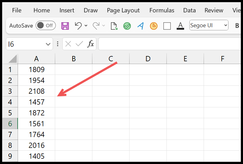
Steps to Apply Conditional Formatting to an Entire Column
- First and foremost, select the entire column with the keyboard shortcut (Ctrl + Space) or click on the column header.

- Afterward, go to the Home Tab > Conditional Formatting > Highlight Cells Rules > Greater Than.

- Now, in the Greater Than dialog box, enter 1500 in the “Format cells that are GREATER THAN” input box and select the format you want to apply to the cells with the value above 1500.

- Finally, click OK to apply the formatting to the entire column.

Now here, conditional formatting is applied to the entire column, and when you enter a new value at the end, it also checks whether the value is greater than 1500 or not.
If you also select the header cell (like “Amount” in A1), it can get highlighted too, because in a comparison, Excel treats text as greater than any number. To avoid it, use a formula rule instead (Home ➜ Conditional Formatting ➜ New Rule ➜ Use a formula to determine which cells to format) with the following formula, which only checks numbers:
=AND(ISNUMBER(A1),A1>1500)
Highlight the Entire Row Based on One Column
Many times, you want to highlight the whole row of a record when the amount in column A is greater than 1500. For this, select the columns of your data (like A:D), go to New Rule ➜ Use a formula to determine which cells to format, and enter the formula below. The $ before A keeps the check on column A for every cell in the row:
=AND(ISNUMBER($A1),$A1>1500)
Write the formula for the first row of your selection. If you start the selection from row 2, use $A2 instead of $A1.

Using a Table Instead of an Entire Column
There’s no problem when you apply conditional formatting to an entire column, but if you use an Excel Table (Ctrl + T to apply), you can make it dynamic. It will extend the conditional formatting once you enter a new value.

In the above example, conditional formatting only applies to the range A1:A100. However, as we have applied the Excel Table to the data, when you enter a new value to extend the data range, it also extends the conditional formatting along with it as well.

Both methods work great; you can choose the one that suits your requirement.
Apply Conditional Formatting to the Entire Row
If you want to apply conditional formatting to the entire row, you can use the same steps we used in the above example.
All the steps are the same; you need to select the entire row first and then apply conditional formatting to it. And to select an entire row, click on the row header or use the keyboard shortcut Shift + Space.
Frequently Asked Questions
Does conditional formatting on an entire column slow down Excel?
A simple rule like Greater Than is fine. But formula rules on full columns are checked for over a million cells, which can make a big file slow. In that case, apply the rule to an Excel table or to a fixed range like A2:A5000.
How do I see which range a rule applies to?
Go to Home ➜ Conditional Formatting ➜ Manage Rules. The “Applies to” box of each rule shows its range, like =$A:$A for the entire column A, and you can change it there.
How do I remove conditional formatting from an entire column?
Select the column, then go to Home ➜ Conditional Formatting ➜ Clear Rules ➜ Clear Rules from Selected Cells.

Written by
Puneet Gogia
Microsoft MVP — Excel · Founder, Excel Champs
Twelve years of teaching Excel, and a decade before that using it as a data analyst. Every tutorial here is written from a file I actually built.