This Tutorial is Written by Puneet Gogia (Microsoft Excel MVP) was last updated on 01-Feb-2026

In Excel, when you have data, most of the time you don’t have serial numbers by default. However, adding serial numbers to the data makes it much easier to manage. When you assign a serial number to each entry, every entry becomes unique, and it becomes easier to identify any specific entry using its serial number.
When you’re using Excel, adding serial numbers is quite easy. With the introduction of a few new methods, it has become even easier to add serial numbers to your data. You can also use different methods to generate automatic serial numbers, so whenever you add a new entry to the data, serial numbers are added automatically for all newly updated entries.
In this tutorial, we are going to explore all the methods available in Excel to add serial numbers, including the method that allows you to automatically add serial numbers to the data.
Is there any benefit of using Serial Numbers in Data?
Yes, there are quite a few benefits of using serial numbers in your data. One of the biggest benefits is that serial numbers give a unique identity to each entry in the dataset.
They also allow you to filter entries easily based on the serial number. For example, if you want to filter the first 50 entries, you can simply apply a filter and select the first 50 or even the last 50 entries. This makes filtering and analyzing data much more convenient.
In addition to that, serial numbers instantly give you a clear count of your data. If you have, say, 500 entries, you can immediately identify that there are 500 records just by looking at the serial numbers.
One of my favorite benefits of using serial numbers is that they allow you to flip your data instantly. Whether you’re using normal serial numbers or date serial numbers, serials make sorting extremely easy.
For example, if your data is sorted from 1 to 500, you can instantly reverse the order and sort it from 500 to 1. This flexibility is one of the biggest advantages when working with data and analyzing it, and it’s a benefit that I personally find extremely useful.
Simple Formula to Add Serial Numbers in Excel
If you ask me the easiest way to add serial numbers in Excel, I will say it’s by using a formula and then dragging that formula down. This is the simplest method to add serial numbers.
All you need to do is select the first cell from where you want to start your serial numbers and enter 1 in that cell. When you press Enter, the active cell moves down to the next cell. In this second cell, enter a simple formula that refers to the cell above where you entered 1. In my case, that cell is A2, and then add 1 to it using the addition operator. When you press Enter, you’ll see 2 in the second cell.
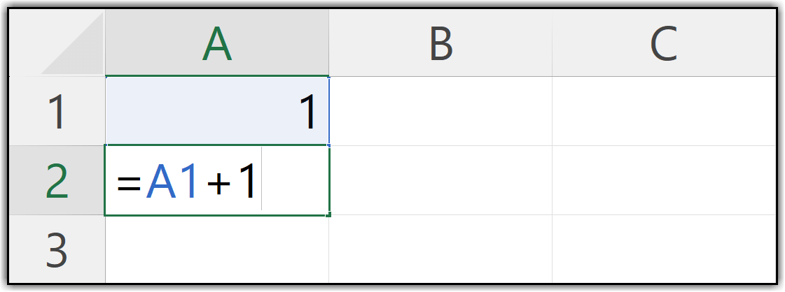
After that, use the fill handle to drag this formula down to the number of cells where you want serial numbers. For example, if you want 10 serial numbers, simply drag the formula down until the last cell shows 10.

That’s the easiest way to add serial numbers in Excel.
Serial Numbers using Fill Handle
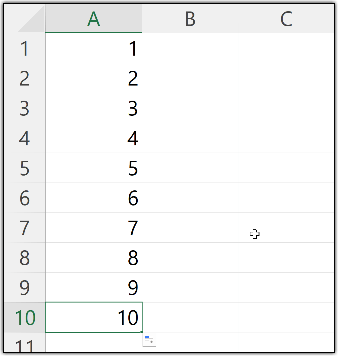
Even if you don’t want to use a formula to get serial numbers, there’s another simple way to do it. You just need to enter 1 in a cell and then drag that value down to the cells where you want serial numbers.

When you do this, you won’t get serial numbers immediately, instead, you’ll see the value 1 repeated in all the selected cells. After dragging, you’ll notice a small drop-down at the end of the range called Auto Fill Options.

When you click on this drop-down, you’ll see a few additional options. From there, select Fill Series. The moment you choose this option, all the repeated 1s in the range are converted into a sequence of numbers, which become your serial numbers. We’ll cover the Fill Series option in more detail in a later method.
Using the Sequence Function to Add Serial Numbers Automatically (The Best Way)
With the new SEQUENCE function, you can easily add serial numbers in one go. For example, if you want to insert 1,000 serial numbers into your data, you just need to write a simple formula using the SEQUENCE function, and it will add all those serial numbers for you automatically.
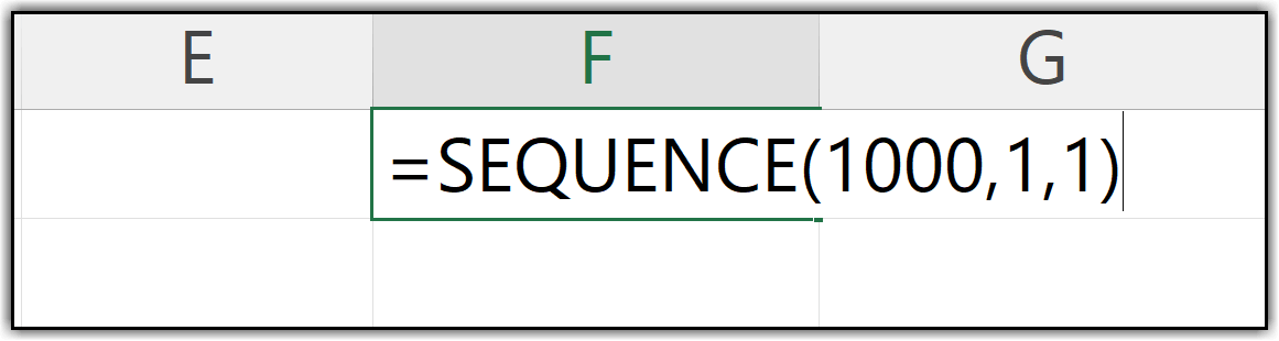
=SEQUENCE(1000,1,1)The idea of using the SEQUENCE function here is to generate a sequence of numbers, and that sequence becomes our column of serial numbers. When you enter the SEQUENCE function in the cell from where you want to start your serial numbers, the first argument is rows. In the rows argument, you need to specify the total number of serial numbers you want.
For example, if you want 1,000 serial numbers from 1 to 1,000, you need to enter 1,000 here. After that, the second argument is columns, where you can enter 1, or you can also skip this argument. The third argument is start, where you specify the first serial number. So, if you want to start your serial numbers from 1, you will enter 1 here.
Once you enter 1 and close the function, it will start from 1 and generate 1,000 serial numbers automatically.

The best part of using the SEQUENCE function is that you have full control over how you want to add your serial numbers. For example, if you want to generate serial numbers with a gap of one number, such as 1, 3, 5, you can specify that value in the step argument.
=SEQUENCE(1000,1,1,2)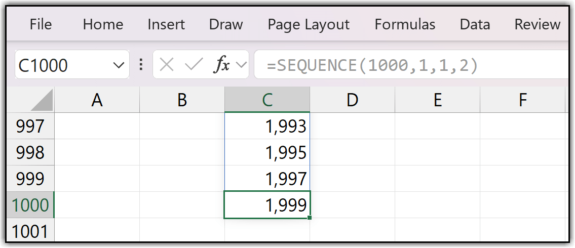
Let’s say you want to add a letter or some text along with the serial numbers. In that case, you can use simple text with a concatenate method along with the SEQUENCE function, and it will return that letter or any text you want together with the serial numbers.
In my case, I’m using the letter S and a hyphen before the serial number, so this formula works accordingly. The formula will look something like the one shown below.
="S-"&SEQUENCE(1000,1,1,2)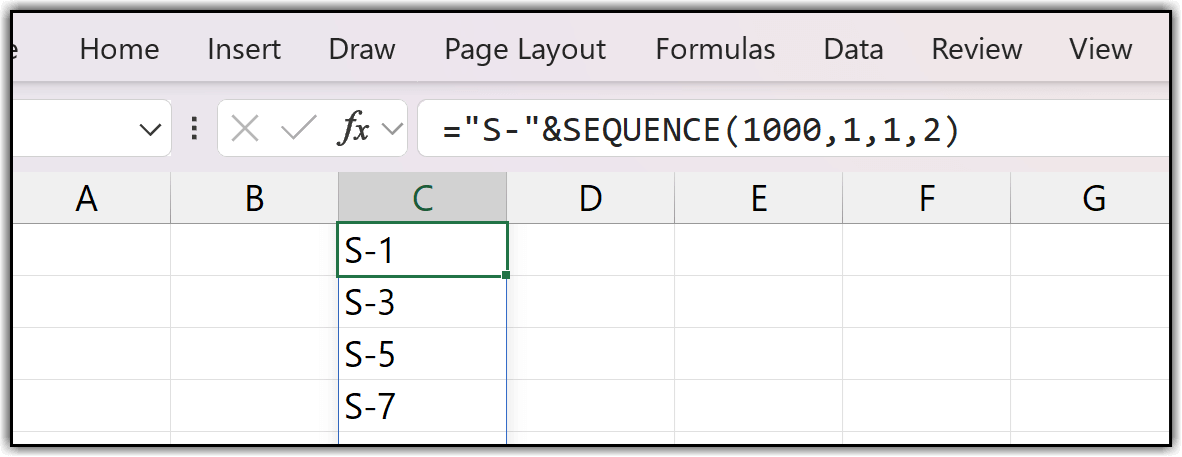
If you want to connect your SEQUENCE function with a different column to test whether a value exists in that column, you can do that as well. For example, let’s say you want to add serial numbers in column A, and you have your actual data in column B. Now, you want to add serial numbers only when a value is present in column B.
Suppose you have three entries in column B and you want serial numbers from 1 to 3. The SEQUENCE function provides a dynamic method that not only inserts serial numbers but also checks the second column, which is column B, and then adds serial numbers based on the entries there.
In my example, I’m using the SEQUENCE function along with the COUNTA function, where the reference range is column B from B2 to B1000. Now, when you enter one more value, say, a fourth entry, in column B, the serial numbers automatically expand from 3 to 4.
=SEQUENCE(COUNTA(B2:B1000))Use Fill Series to Generate Serial Numbers in Excel by Dragging
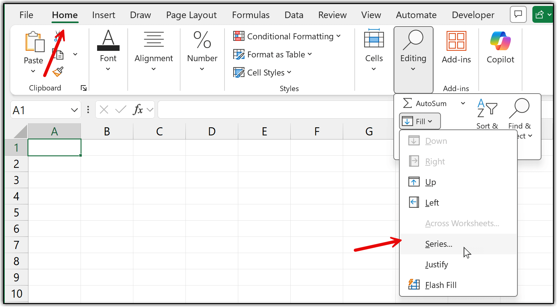
In Excel, there is another way to insert serial numbers instantly, and that is by using the Series option. If you go to the Home tab, you’ll find a drop-down called Fill, and within that Fill drop-down, there is the Series option. To use this option, you first need to enter the initial serial number in a cell. For example, if you want to start from 1, simply enter 1 in a cell.
After that, go to the Home tab again, open the Fill drop-down, and select the Series option.
This opens a small dialog box with a few options to choose from. From the Series in section, select the Columns option. In the Step value field, you can change the increment if needed, but here we’ll keep it as 1. In the Stop value field, enter the maximum serial number you want. For instance, if you want serial numbers from 1 to 1000, enter 1000.
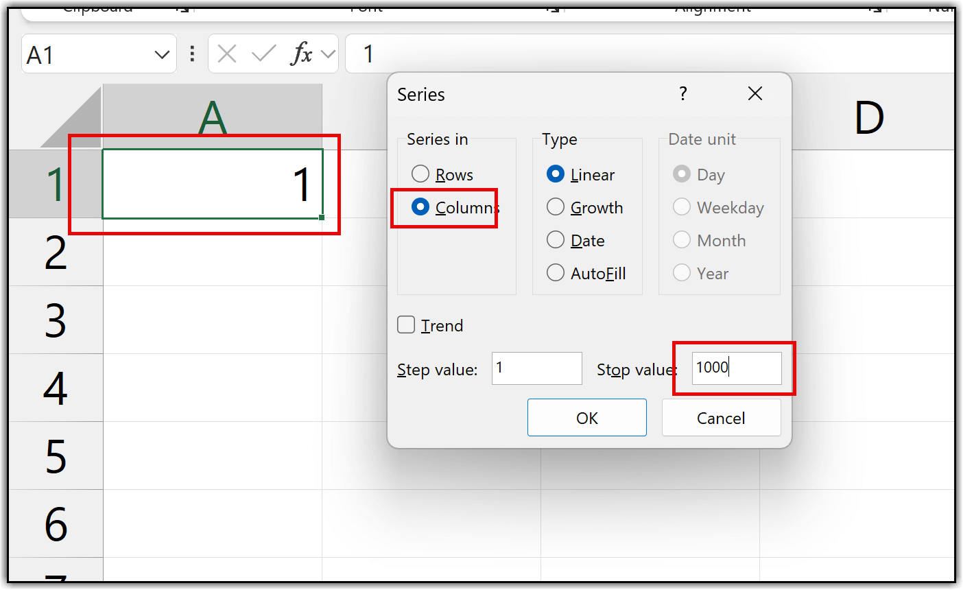
Since 1 is already entered in the selected cell, the moment you click OK, Excel generates serial numbers from 1 to 1000 automatically. This is a simple way to use the Fill Series option to add serial numbers. The only thing you need to keep in mind is that this method is not dynamic. If you want to extend the serial numbers further, you’ll need to use the Series option again.
Using ROWS Function to Add Serial Numbers
If you are using a different version of Excel and you don’t have the SEQUENCE function available, there’s no need to worry. There is another way to write a formula that can generate serial numbers. This method uses the ROW function to add serial numbers.
=ROWS($A$2:A2)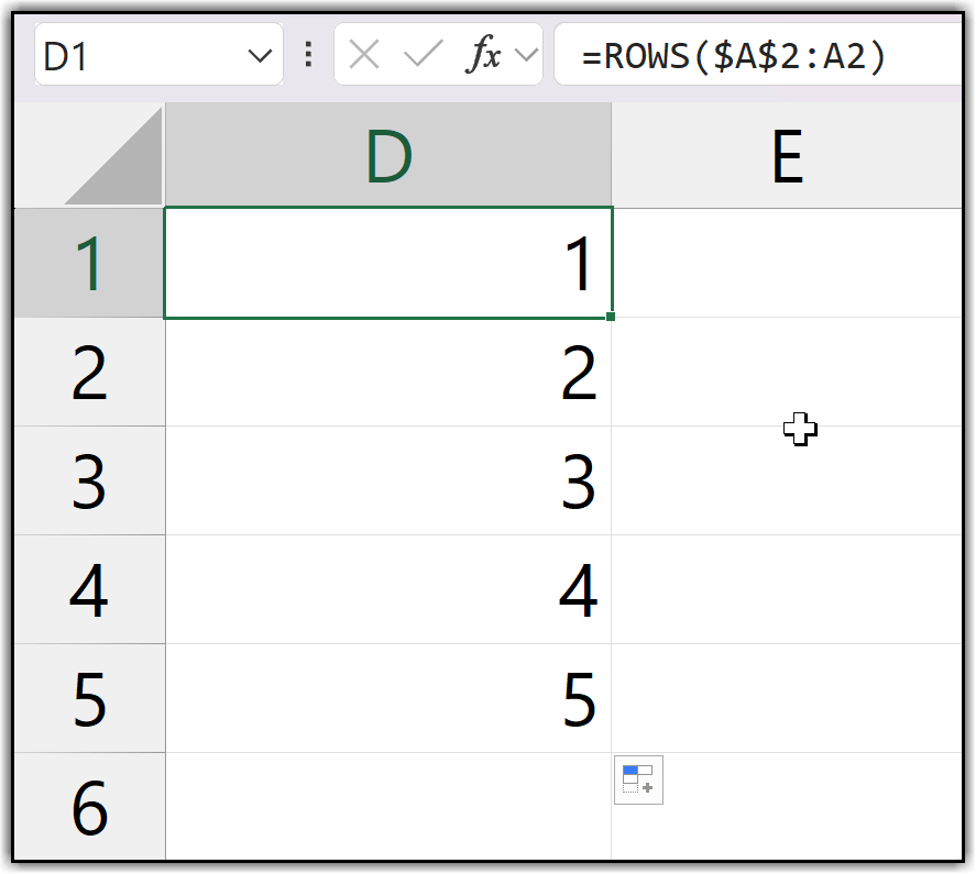
While using this formula, you need to change the cell reference based on where you want to start your serial numbers. In my case, I’m starting the serial numbers from cell A2, which is why I’m using A2 as the reference. But, if you want to start with cell C2, A1, or any other cell, you simply need to change the reference to that specific cell. In the reference, both the first and the last cell will be the same.
The only difference is that in the first cell of the reference, you need to freeze the reference using the dollar sign.
Using an Excel Table to Automatically Add Serial Numbers
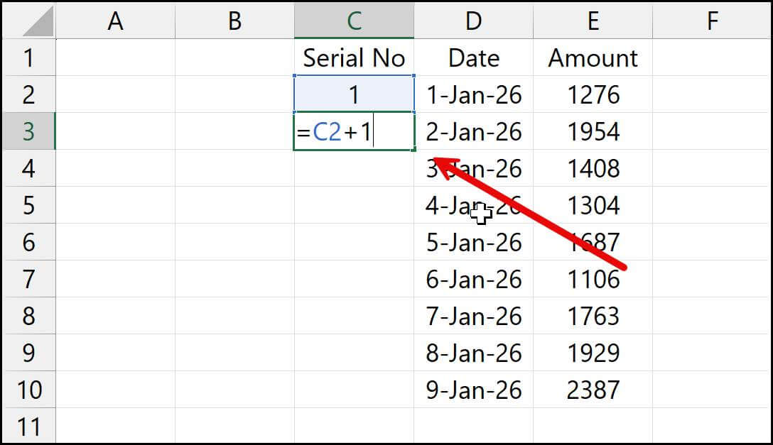
If you convert your normal data into an Excel table, adding serial numbers automatically becomes much easier than any other method. If you look at my sample data here, I have two columns: Date and Amount. First, I’ll add one more column before the Date column and name it Serial Number, or simply Serial No, to define it as a serial number column.
Next, I’ll enter 1 in the first row as the serial number for the first entry. In the second cell, I’ll enter a simple formula that refers to the first serial number cell and adds 1 to it. This gives me serial numbers 1 and 2. After that, I’ll drag this formula down to the last row, which gives me serial numbers from 1 to 9.
Once this is done, I’ll convert the data into an Excel table using the keyboard shortcut Ctrl + T.
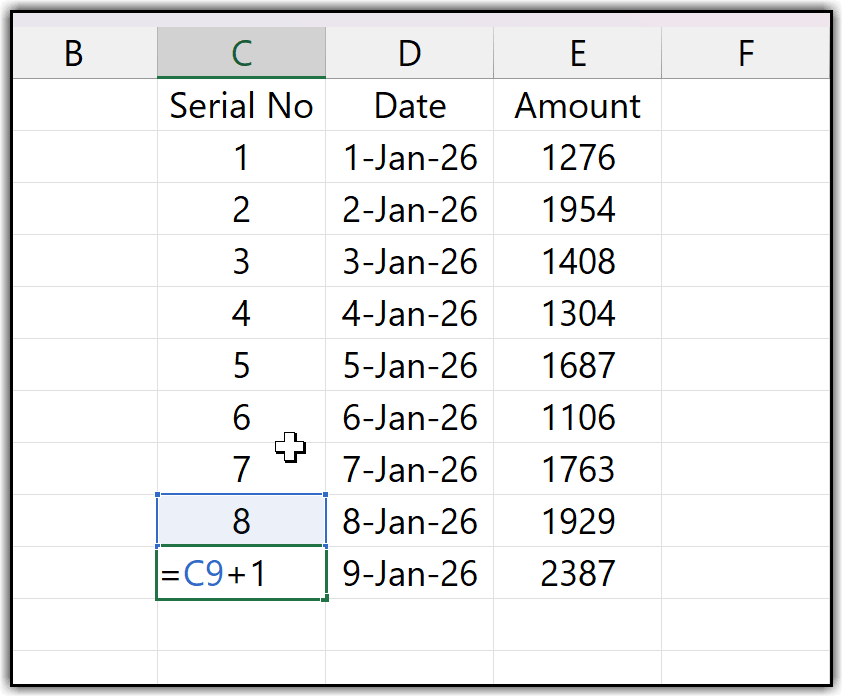
Now I have an Excel table with three columns: Serial Number, Date, and Amount. From this point on, whenever I add a new entry, let’s say I enter the next date, 10 Jan 2026, the moment I press Enter, Excel automatically adds the next serial number, which is 9, without needing to drag the formula down.
This works because Excel tables automatically extend formulas. It’s a one-time setup, and after that, the table will continue to add serial numbers automatically every time you add a new entry.
Creating Dynamic Serial Numbers with Filters
Now let’s talk about a different way of adding serial numbers. Suppose you’re working with data where you apply filters frequently, and you want a dynamic formula that always shows serial numbers starting from 1, even after filtering the data.
For example, I have region-wise data and you want the serial numbers to restart from 1 whenever you filter the data for a specific region. To do this, you first add one more column to your data and name it Serial Number. After that, you use a simple formula based on the SUBTOTAL function to generate the serial numbers dynamically.
=SUBTOTAL(3,B$2:B2)In this formula, the range starts and ends with the same cell, but the first cell is fixed while the second cell is relative. As you drag the formula down, SUBTOTAL keeps the starting cell fixed and keeps extending the ending cell. This creates an expanding range, which gives you the running count of non-blank cells.
This method is not just for generating serial numbers, the real magic of SUBTOTAL happens when you filter your data. When you apply a filter to a particular region, instead of showing serial numbers for the entire dataset, SUBTOTAL recalculates everything based on the filtered results and returns serial numbers only for the visible rows.
For example, if you filter the data for the South region, the serial numbers automatically restart from 1 and continue up to the last visible entry, which in my case is 192. This makes the serial numbers fully dynamic and responsive to the applied filter.
This behavior is not limited to the Region column. It works with any column in your data. So, if you filter the data for a specific state, the serial numbers will again start from 1 and run up to the last entry for that state.
Macro to Add Serial Numbers in one Click
You can also use a VBA code to insert serial numbers in just one click. With the VBA code that I’ve written for you, you can add serial numbers not only as numbers, but also in Roman numerals and alphabets.
For example, if you want serial numbers as numbers, you can select that option. If you want them in Roman numerals or alphabets, you can choose the required option from the message box. All you need to do is add this VBA code as a macro in the Visual Basic Editor and then run it. Once you run the macro, it will insert the serial numbers automatically.
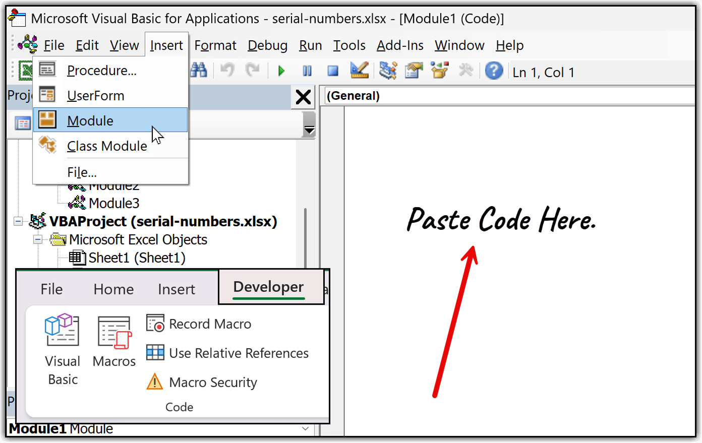
Steps: Developer Tab > Visual Basic > Insert > Module > Paste the Code into the Code Window.
Simple Code to Add Serial Numbers:
Sub AddSerialNumbers()
Dim i As Integer
On Error GoTo Last
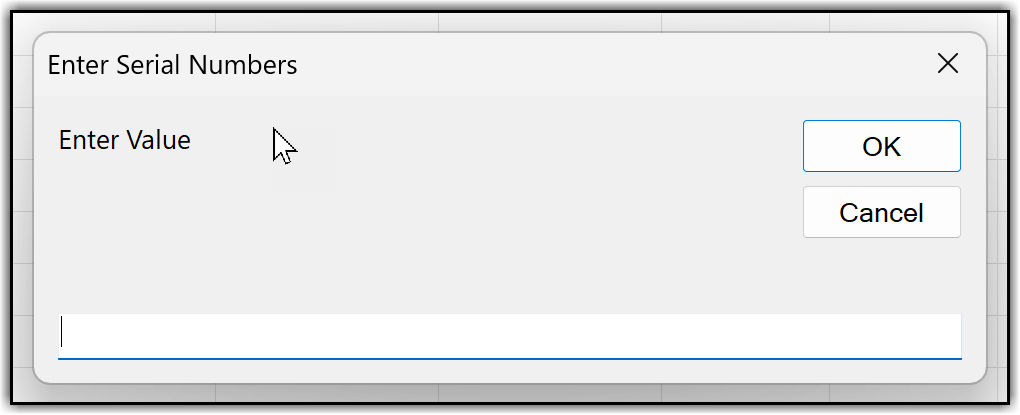
i = InputBox( _
"Enter Value", _
"Enter Serial Numbers")
For i = 1 To i
ActiveCell.Value = i
ActiveCell.Offset(1, 0).Activate
Next i
Last:
Exit Sub
End SubIf you want to add every serial number twice:
Sub AddSerialNumbers2()
    Dim i As Integer

    On Error GoTo Last

    i = InputBox( _
        "Enter Value", _
        "Enter Serial Numbers")

    For i = 1 To i
        ActiveCell.Value = i
        ActiveCell.Offset(1, 0).Activate
        ActiveCell.Value = i
        ActiveCell.Offset(1, 0).Activate
    Next i

Last:
    Exit Sub
End SubAnd if you want to have the option to choose the serial number type:
Option Explicit

Sub AddSerialNumbers_ByChoice()
    Dim rng As Range
    Dim choice As Variant
    Dim i As Long

    'Make sure user selected cells
    If TypeName(Selection) <> "Range" Then Exit Sub
    Set rng = Selection

    'Ask for type
    choice = Application.InputBox( _
        Prompt:="Enter serial type:" & vbCrLf & _
                "1 = Numbers (1,2,3...)" & vbCrLf & _
                "2 = Roman (I,II,III...)" & vbCrLf & _
                "3 = Alphabets (A,B,C...)", _
        Title:="Serial Number Type", _
        Type:=1)

    If choice = False Then Exit Sub 'Cancel pressed

    Application.ScreenUpdating = False

    Select Case CLng(choice)
        Case 1 'Numbers
            For i = 1 To rng.Cells.Count
                rng.Cells(i).Value = i
            Next i

        Case 2 'Roman
            For i = 1 To rng.Cells.Count
                rng.Cells(i).Value = _
                    Application.WorksheetFunction.Roman(i, 0)
            Next i

        Case 3 'Alphabets (A..Z, AA..)
            For i = 1 To rng.Cells.Count
                rng.Cells(i).Value = ColumnLetters(i)
            Next i

        Case Else
            MsgBox _
                "Invalid choice. Enter 1, 2, or 3.", _
                vbExclamation, _
                "Serial Numbers"
    End Select

    Application.ScreenUpdating = True
End Sub

'Converts 1->A, 2->B ... 26->Z, 27->AA ...
Private Function ColumnLetters(ByVal n As Long) As String
    Dim s As String
    s = ""

    Do While n > 0
        n = n - 1
        s = Chr$(65 + (n Mod 26)) & s
        n = n \ 26
    Loop

    ColumnLetters = s
End FunctionAdd Date Serial Numbers in a Column
Sometimes you don’t just need a list of serial numbers, you may also need date serials that start from a specific date and extend for a certain number of days. In such cases, you can use the same methods we discussed earlier; the only thing you need to change is the initial value.
The key thing to understand here is that Excel stores dates as numbers. For example, if you have a date like 1 January 2026, it is actually stored as a number in the background. When you add 1 to that date, Excel automatically returns the next date.
Let’s say you want to start with the date 1 January 2026 and add 30 serial dates, which means you want dates from 1 January to 31 January 2026. The idea here is quite simple.
First, move to the next cell below the starting date and enter a simple formula. Use an equals sign, refer to the cell where you have the first date, and then add 1 to it. This gives you the next date after 1 January 2026, which is 2 January 2026.
After that, use the fill handle to drag this formula downward to the cell where you want the last date. In this case, since you need dates up to 31 January 2026, you just drag the formula down until that date appears. This way, you can generate all the serial dates in one go.
Now, let’s look at another method.
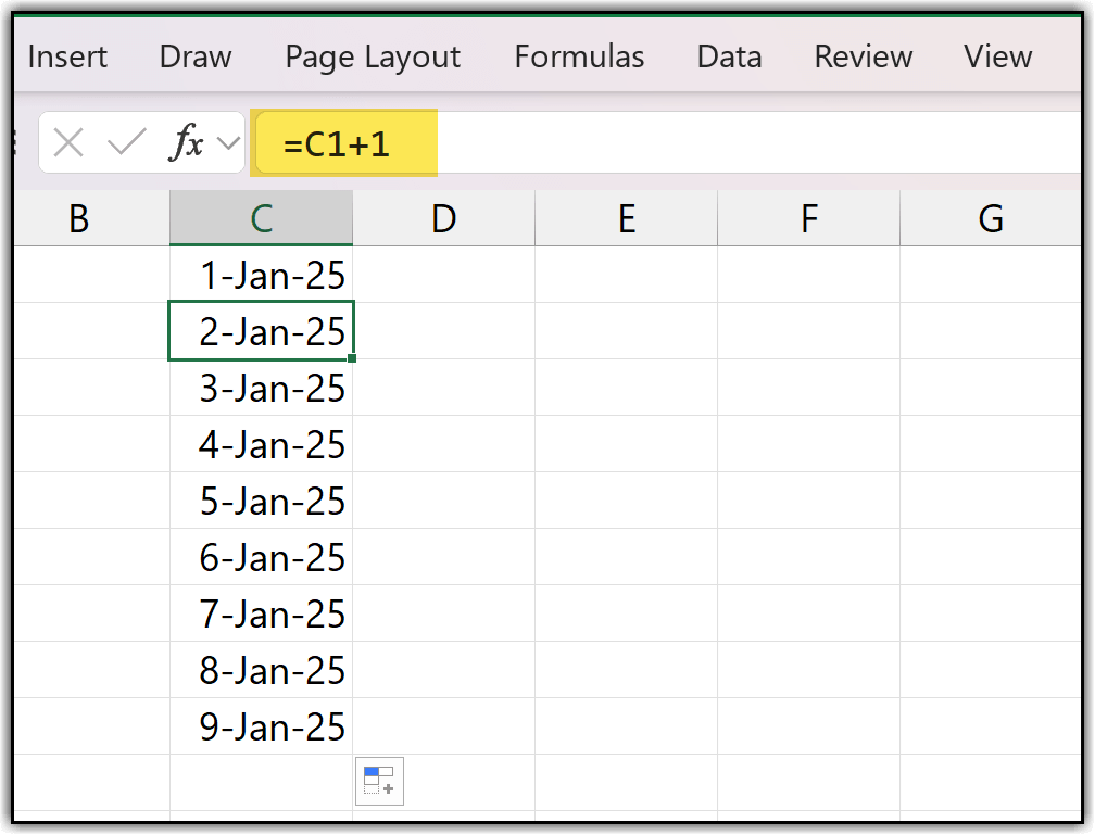
First, enter the starting date that you want. After that, click on the bottom-right corner of the active cell where the first date is entered. Then, press and hold the mouse button and drag the date down to the cell where you want the series to end.
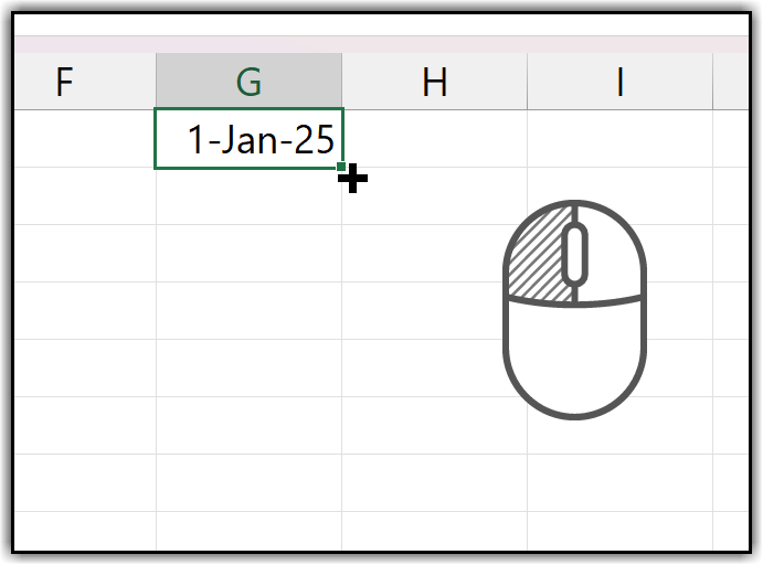
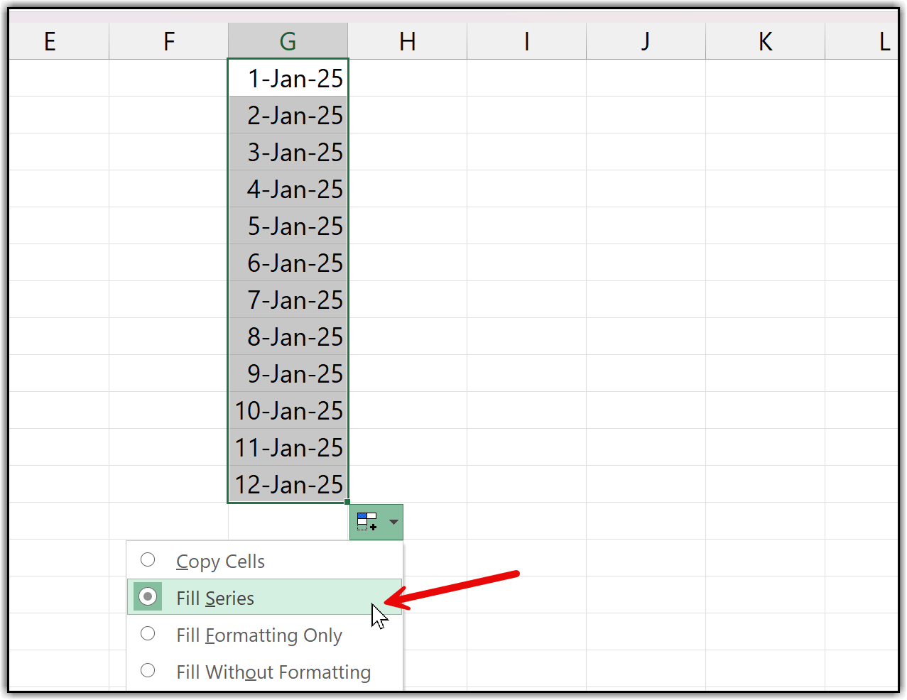
For example, if I drag it down for 12 more cells, Excel shows a small drop-down menu. In that drop-down, there is an option called Fill Series. When you click Fill Series, Excel fills the cells with consecutive dates.
In my case, I start with 1st January 2025. When I drag the date downward and choose Fill Series from the drop-down, Excel fills the cells with serial dates up to 12th January 2025
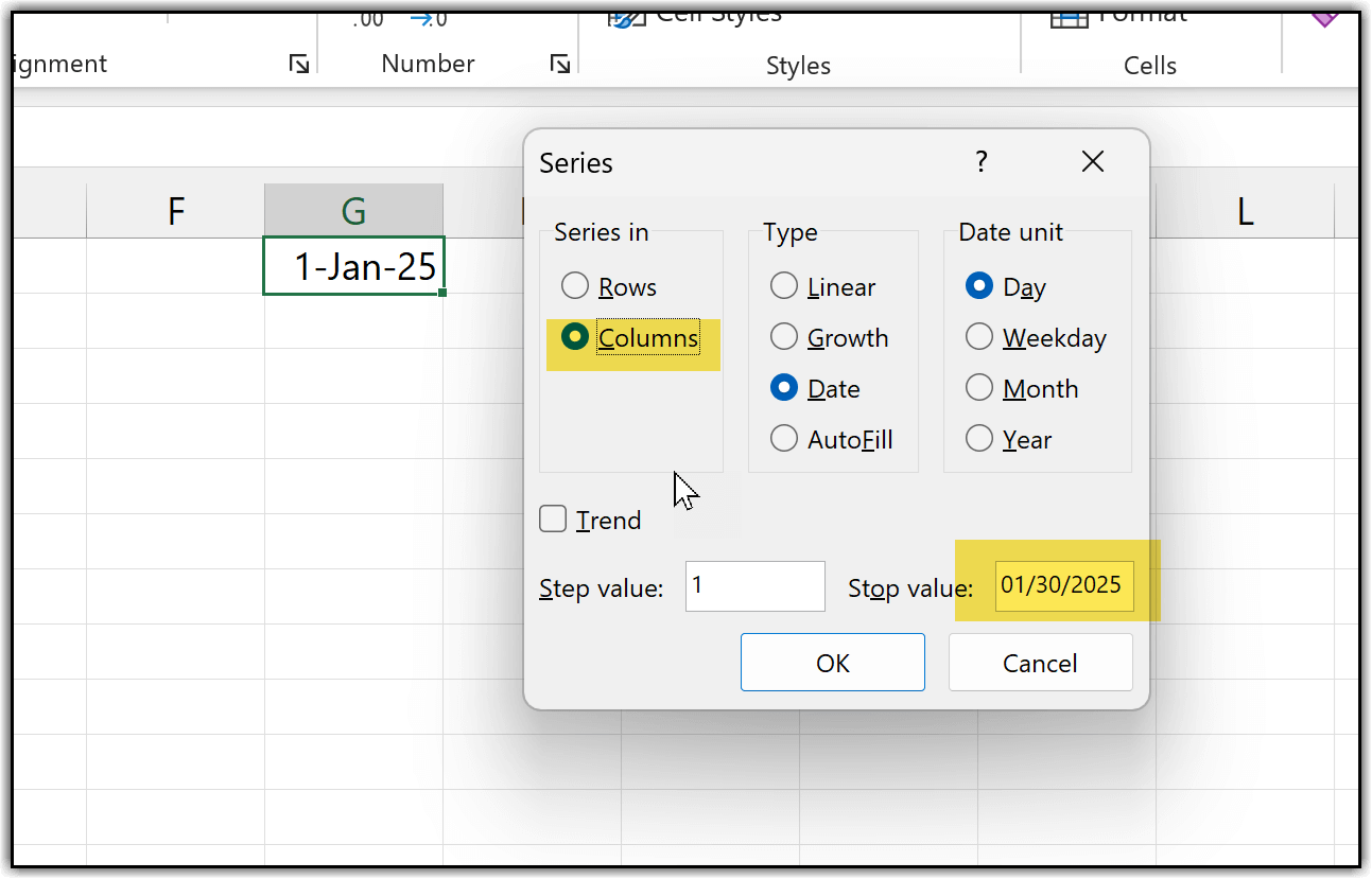
Apart from this method, you can also use the Fill Series option to get serial dates instantly in your worksheet. The idea is the same, you need to have the first date entered in a cell. In my case, I have 1 January 2026, and I want 30 more dates.
To do this, go to the Home tab, click the Fill drop-down, and then select Series. In the dialog box, choose Columns under the Series in option. The Date type is already selected, and the Date unit is also set to Date. In the Stop value, instead of entering the count of serial numbers or serial dates, you need to enter the actual date. Here, you must use a specific date format, which is mm/dd/yyyy. So, I’ll enter 01/31/2026 as the stop value. When you click OK, Excel generates dates up to 31 January 2026 automatically.
Is there a keyboard Shortcut to Insert Serial Numbers?
By default, there is no built-in keyboard shortcut in Excel to insert serial numbers. But you can build a workaround that assigns a keyboard shortcut, so you can insert serial numbers quickly just by using that shortcut.
To do this, the first thing you need is a macro that can insert serial numbers for you, within a specific range, for example from 1 to 1000. You then need to add that code into the Visual Basic Editor. You’ve already learned this in the earlier section where I shared three different macros to insert serial numbers, so the setup is the same here as well. We just need a macro for this method too.
Option Explicit

Sub AddSerialNumbers_FromSelectedCell()
    Dim startCell As Range
    Dim n As Variant
    Dim i As Long
    'Start from selected cell
    If TypeName(Selection) <> "Range" Then Exit Sub
    Set startCell = ActiveCell
    'Ask how many serial numbers
    n = Application.InputBox( _
        "How many serial numbers do you want to add?", _
        "Add Serial Numbers", _
        Type:=1)
    If n = False Then Exit Sub 'Cancel
    If CLng(n) <= 0 Then Exit Sub
    'Fill serial numbers downward
    For i = 0 To CLng(n) - 1
        startCell.Offset(i, 0).Value = i + 1
    Next i
End SubYou can use the macro I shared above. Just go to the Developer tab, click Visual Basic, insert a new Module, paste the code into the code window, and then close the Visual Basic Editor. Now, once you add this code to the Visual Basic Editor, the next step is to add this macro to the Quick Access Toolbar. When you add the macro there, you can run it using a simple keyboard shortcut with the Alt key. That’s the workaround we’re going to use here.
Now, once you add this code to the Visual Basic Editor, the next step is to add this macro to the Quick Access Toolbar. When you add the macro there, you can run it using a simple keyboard shortcut with the Alt key. That’s the workaround we’re going to use here.
From here, you need to go to the File tab and click on Options.
When you do that, the Excel Options dialog box opens. In this dialog box, go to Quick Access Toolbar. Here, you’ll see two sections: one that shows all the available commands, and another that shows the commands already added to the Quick Access Toolbar.
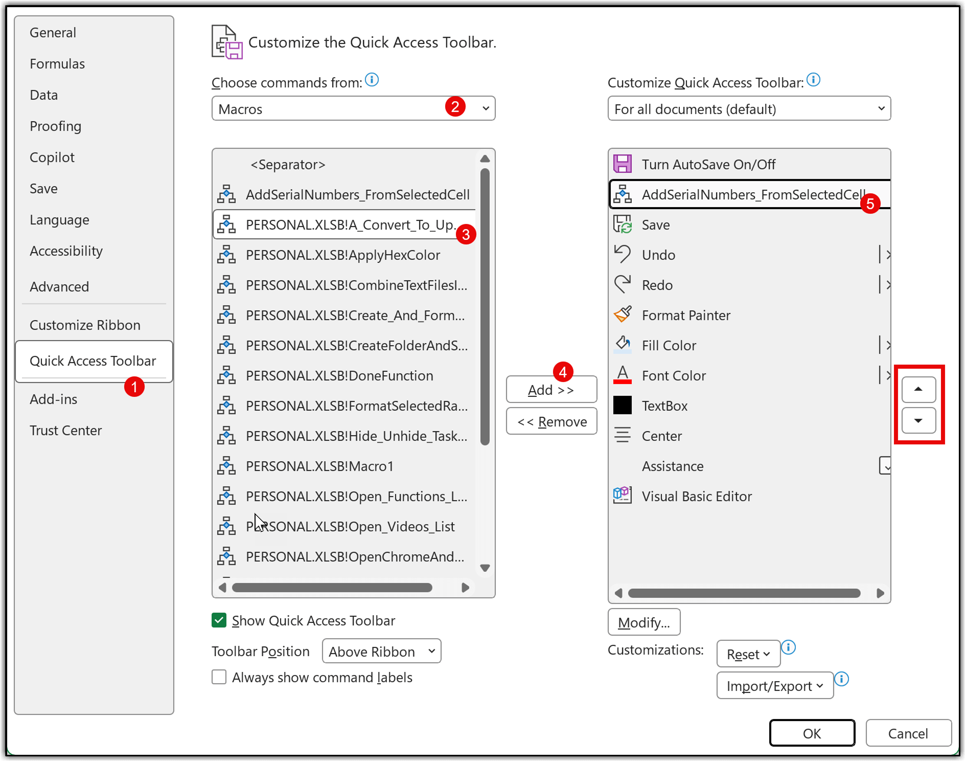
Now, from the Choose commands from drop-down, select Macros. This will display all the macros available in your workbook. At this point, I would also suggest learning more about the Personal Macro Workbook, which allows you to use VBA code across all workbooks instead of just one.
In my case, I already have a Personal Macro Workbook, and the code is saved there, which is why I’m selecting the macro from it. Next, select the macro you want to use and click Add. The macro is now added to the Quick Access Toolbar. To make it easier to use with the Alt key, you should move this macro to the first, second, or third position.
This position decides the shortcut key you’ll use.
After that, select the same macro on the right side and click Modify. Here, you can assign an icon that helps you identify this macro as one used for serial numbers.

You can choose any icon you like, here, I’m selecting a green icon. Click OK, and then click OK again to close the dialog box.

Now, if you look at the Quick Access Toolbar, you’ll see the green icon added there. When you press the Alt key on your keyboard, Excel displays numbers on the Quick Access Toolbar.
Since this macro is in the second position, pressing Alt + 2 runs the macro. When the macro runs, it asks how many serial numbers you want to add. If you enter 1000, it inserts 1000 serial numbers starting from the selected cell. This way, you can use a keyboard shortcut every time you want to insert serial numbers.
Once again, I recommend learning more about the Personal Macro Workbook, as it allows you to store useful VBA codes and use them across all your Excel workbooks.
how to insert 4 columns in between sl.no. 1 to 800 for example sl.no.1 4 empty columns, sl.no.2 4 empty columns, sl.no.3 4 empty columns, this through out the 800 sl.nos
i want to put serial no as below data in automatic (colon A having s/n, B having group data but i need sn in group data wise
1 HS Code
24031100
24031100
24031100
2 HS Code
22 02 99 90
3 HS Code
24031920
24031920
24031920
4 HS Code
24022010
5 HS Code
24021000
24021000
24021000
Dynamic Serial Number method good find.
Also Learnt usage of Row and CountA function in Serial number from this. Thank you 🙂
Thanks a lot for your explanations! it really helped me..I personally like method 3 and 5.
What formula will be use for this type of numbring
S.N. QUALITY
1 2/60 ERI
1 10 S SLUB COTT
1 25S ACRLYIC
2 2/60 ERI
2 2/20 COT
2 10 COTTON
2 2/40 COTTON
3 2/60 ERI
3 2/20 COT
3 10 COTTON
3 2/40 COTTON
4 2/20 COTTON
4 2/60 ERI
4 25 S ACRLYIC
did you get an answer in regards to this?
I am not clear with your Method #10. can you explain clearly?
I have a serial numbers as A,B,C,D,…Z. If I delete one of the row, the series of A,B,C,D,E…Z should not be changed. it should again shows A,B,C,D,E,…..Z. please help…its urgent.
I WANT TO ADD SR NUMBERS AS 1(18-19) AND THAN 2(18-19) IN A COLUMN BUT BECAUSE OF () I AM NOT ABLE TO ADD SERIAL NUMBERS PLS HELP
You need to use ROW function and then add (18-19) as a test so if I have to insert serial number in cell A1 then the formula would be =ROW()&”(18-19)”
How to add Serial no. having figure more than 15 digits, like 89080068770002819
Give me a better example. what do you mean by 15 digits? 🙂
what the formula for method 10
awesome work !
excel
I often use MAX to achieve automated numbering, with cell formatted as a number ending in decimal point (“#,##0.”), with a dependency on the cell to the right having a value in it.
For example
With Row 1 having column headings, I would have the following formula in call A2 –
=if( $B2 = “” , “” , max( $A$1:$A1) + 1
which can then be dragged / copied down to the bottom of the sheet or area you need it to apply to. Useful to apply step by step documentation of steps in a process, where blank lines between any steps do not get numbered.
I need to insert automatic serial no.s like :
TK001
TK002
TK003 ….and so on.
with condition that when there is some entry in the next coloum even then this serial no. has auto entered.
DID YOU GOT IT ? I AM SEARCHING FOR THE SAME
i want to get a series like 1,1,2,2,3,3,4,4,5,5,.. and so on. How to do that?
Sub AddSerialNumbers()
Dim i As Integer
On Error GoTo Last
i = InputBox(“Enter Value”, “Enter Serial Numbers”)
For i = 1 To i
ActiveCell.Value = i
ActiveCell.Offset(1, 0).Activate
ActiveCell.Value = i
ActiveCell.Offset(1, 0).Activate
Next i
Last:
Exit Sub
End Sub
Let’s say your sequence begins in cell A2.
In cell A2, enter a 1
In cell A3, enter this formula:
=IF(COUNTIF($A$2:A2,A2)=1,A2,A2+1)
Use the fill handle to drag that down as far as needed.
Please help
To get serial chace
How to do that please help
hii
i want to make auto fill column like 3 9 27 81
Multiply with three and drag down.
Its owesome Yaar
Thanks for your words. 🙂
I often use COUNTA(A$1:A1) to add serial number.for filering i’d love SUBTOTAL(3,B$1:B1)
Thanks for sharing.
The other day I learned the following:
– in Cell A1 type the number 1
– while holding down CTRL button, use Fill Handle on bottom right hand corner of cell A1 and drag down
– you will see the numbers filled in sequential order as you drag down
Thanks Derek
Well,
this is my favorite as it works with filtering:
=subtotal(3,a$1:a1)
Wow, MMA,
Thanks for sharing.
Do I miss something here? I have put the subtotal function in A1 and copied it down. What I get is 0 (zero) in all my cells. I use the norwegian version and the 3 points to COUNTA, is that correct?
formula should be =SUBTOTAL(3,B$1:B1)