Format Millions with One Decimal in Excel

Sometimes, when you work with data and have large numbers, it is hard to read the numbers. Even the other person cannot read the number and make mistakes while working with data.

Let’s say you have a number, amount, or currency in millions; in Excel, you can convert these numbers into single-digit numbers with one or two decimal to show as millions.

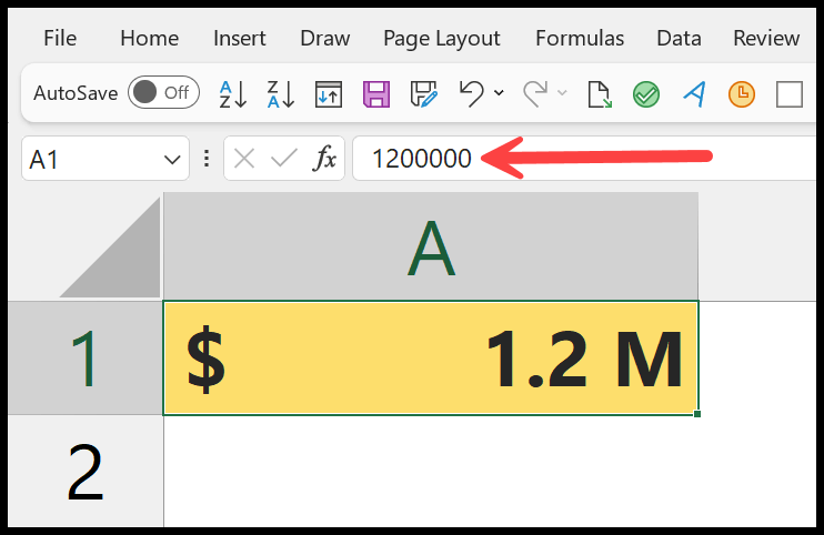
In the above example, we have the same number in both cells, but the readability is way better in the second one. This custom format shows one million as a single number and we have one decimal after that to present the rest of the part.

Using 1200000.0 as 1.2 M makes it easily readable. It is specifically beneficial when dealing with financial data so users can easily read it. Apart from custom format, there are multiple ways to do that, and in this tutorial, we will learn all those methods in detail.

Using Custom Formatting to Convert Format Million with a Single Decimal

As I said, the best way to do this is to use custom formatting. This is because custom formatting doesn’t change the values in the cell or range but applies formatting to show the number in a particular way. Here are the steps to follow:

1. Select the cell or the range of cells where you have values that you want to show a million with a single decimal.
   
2. After that, right-click with the mouse and go to the “Format Cells…”. You can also use the keyboard shortcut key (Ctrl + 1) to open the format cells dialog box.
   
3. Now, in the Format Cells dialog box, go to the Custom, and in the “Type” input bar, enter the format ($* 0.0,, “M”).
   
4. Finally, click the “OK” button to apply the formatting.

When you click OK, it converts the cell’s formatting with the desired formatting million with one decimal.

You can see in the formula bar that the cells’ value is exact; there is no change in it. The only change is in the formatting of the cell.

In the custom format, we have used “M” as a suffix, and you can change it the way you want; you can use “Mil” instead of “M”. Apart from this format, you can also use the below formats for the apply the custom formatting:

• $* #,##0.0,,"M"
• #,##0.0,,"M"

And, if you want to use any other currency symbol, you can replace the dollar with that symbol. Let’s if you want to use Indian Rupee, you can use formatting like below:

• ₹* #,##0.0,,"M"
• ₹* 0.0,, "M"

Note – If you have multiple cells, a row, or a column to apply the custom formatting, you must select the row or the column entirely and then open the custom format dialog box. You can also use the Format Painter to apply the formatting from one cell or range to another cell or range.

Other Methods to Show Millions with One Decimal

Custom formatting is the best way to do this as it doesn’t change the value of the cell. But there are a few more ways to modify the value of the millions to a number with one decimal.

Note — All the methods you will learn ahead convert a number into text when converted into a million with one decimal number.

Using the ROUND Function

With the round function, you can write a simple formula to divide the original number with 1000000, concatenate an “M” with the number, and show it as a single number.

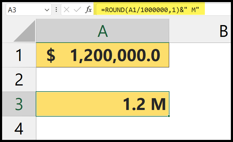
=ROUND(A1/1000000,1)&" M"

In the round function, there are two arguments to define:

• number – In this argument, we divide the original number by 1000000 to convert it into a single-digit number.
• num_digits – In this argument, we have used 1 to tell the function that we need only one decimal in the result.

You can use an ampersand to get the “M” and the number as a suffix.

Using the TEXT Function

The same thing can be achieved with the TEXT function. In the TEXT function, you can specify the format you want for the, and then TEXT will convert it into that and get the result in the cell.

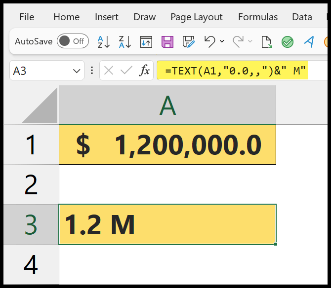
=TEXT(A1,"0.0,,")&" M"

You can use an ampersand to get the “M” as a suffix.

In the TEXT function, in the first argument, we refer to the cell where we have the original number, and then in the “format_text” argument, we use the format (0.0,,).

And in the end, you can use an ampersand to get the “M” along with the number as a suffix.

Use Paste Special to Convert Millions into a Single Number with One Decimal

With the help of the paste special option, you convert large numbers into small numbers. Let’s you want to convert the same number which we have used in the earlier examples:

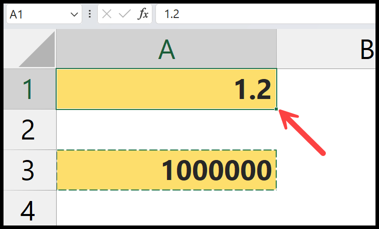
1. First, enter “1000000” in a single cell and select that cell.
   
2. Now, use the keyboard shortcut Ctrl + C to copy the value from the cell, or you can use the right-click.
   
3. Next, you must select the cell where you want to convert the value into a million with a single decimal. And then, right-click and open the paste special option.
   
4. After that, in the paste special dialog box, click on the “Divide” and then click “OK” to perform the calculation.
   

Once you click OK, it divides the value in the cells by one million, which you have copied from the cell earlier. And the value I have in the cell now is 1.2, which means 1.2 million.

Which Method is Best?

Custom formatting is the best method to format millions with one decimal. This is because when you apply custom formatting, it doesn’t change the value in the cell; it just changes the formatting.

On the other hand, all the other methods we have used convert the number into text, making it hard to use the data further, like when you need to create a change for this.