

Select the range, go to Home → Conditional Formatting → New Rule → Use a formula to determine which cells to format, and combine the conditions in one formula. =AND(A2>=700,A2<=1500) formats a cell only when both conditions are true; =OR(A2<700,A2>1500) formats it when either one is. Click Format, choose a colour and click OK.
Write the formula for the top-left cell of your selection. If you selected A2:A20, the formula refers to A2 and Excel adjusts it for every other cell. A formula that points at a different row shifts the highlight up or down.
To test conditions in two columns, lock the columns with $: =AND($B2="a",OR($A2<700,$A2>1500)). Apply it to A2:A20 to colour only the values, or to the whole table to colour entire rows. The rule needs only the logical test, so wrapping it in IF(…,TRUE,FALSE) adds nothing.
For a different colour per condition, create one rule for each, for example Highlight Cells Rules → Greater Than 1500 and Highlight Cells Rules → Less Than 700. Where two rules are true and their formats clash, the rule higher in Conditional Formatting → Manage Rules wins; tick Stop If True on a rule to stop the rules below it applying to that cell.
If the highlights look wrong, check for numbers stored as text. Excel treats any text as greater than any number, so a text value passes A2>1500 and fails A2<700 without showing an error. Text tests such as $B2="a" ignore case but fail on a trailing space.
In Excel, you can use conditional formatting to apply multiple conditions on a single cell or a range of cells. And there are two ways to do that:
- Apply the rule twice.
- Or use a formula to test two conditions at the same time.
In this tutorial, we will learn to use these methods in detail.
Multiple Conditions in Conditional Formatting (Two Conditions)
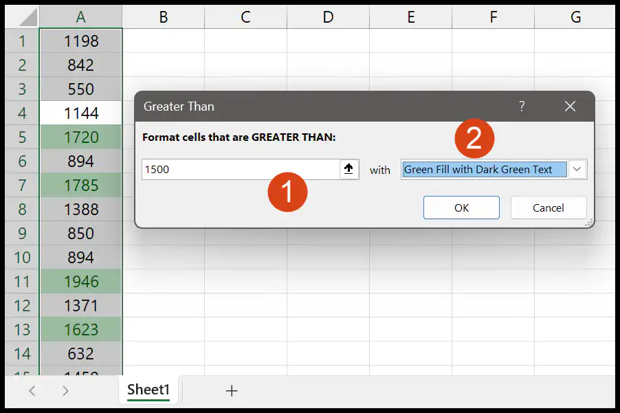
- First, select the range of cells where you want to apply the conditions and go to Conditional Formatting > Highlight Cells Rules > Greater Than.

- From here, in the dialog box, enter 1500 and select formatting to apply to the cells greater than 1500. Once you do this, click OK to apply the rule.
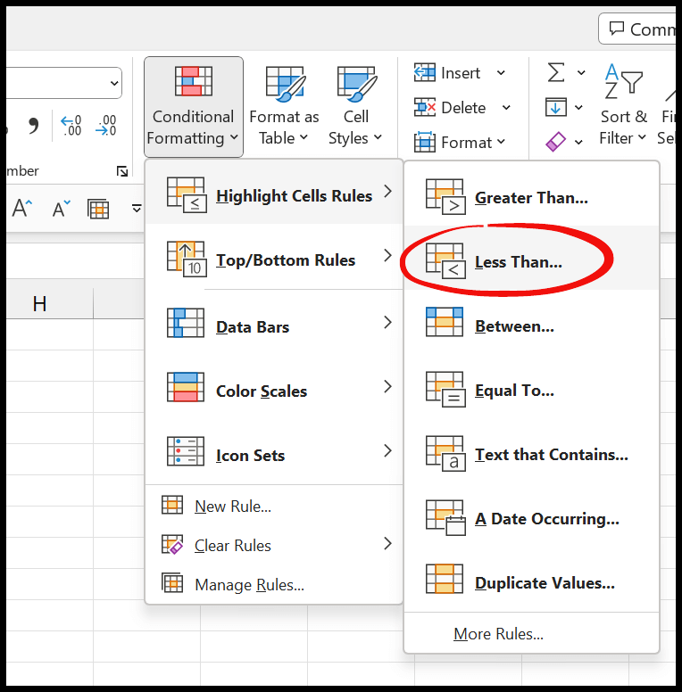
- Again, go to Conditional Formatting > Highlight Cells Rules > Less Than.
- After that, in the dialog box, enter 700 and select the formatting you want to apply to the range. Once you do that, click OK to apply the rule.
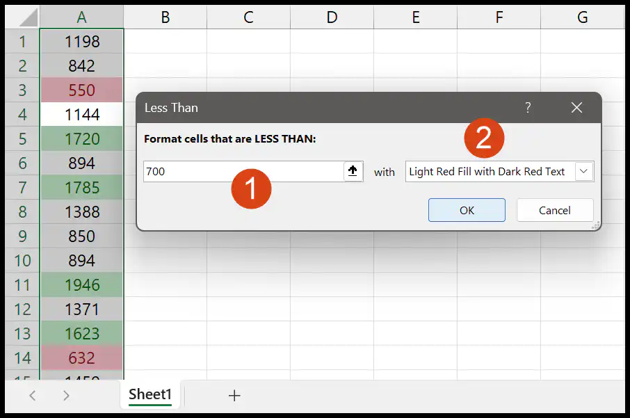
Now here you have two conditions applied to the same range of cells. In the first condition, it highlights the cells where the value is greater than 1500; in the second condition, it highlights the cells where the value is lower than 700.
Each rule can have its own color. If two rules ever apply to the same cell, the rule higher in the list (Home > Conditional Formatting > Manage Rules) wins where their formats clash. You can change the order there, or tick Stop If True to stop checking the rules below it.
Multiple Conditions in Conditional Formatting (Single Formula)
In this method, you use a formula to test two conditions in a single rule.
- First, select the range of cells, and go to Conditional Formatting > New Rule.
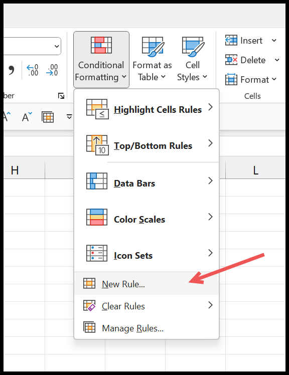
- From the dialog box, click on “Use a formula to determine which cells to format”.
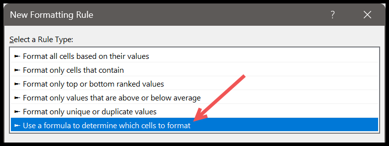
- After that, in the formula input bar, enter the formula =IF(OR(A1>1500,A1<700),TRUE,FALSE), and then click on the “Format…” button to specify the format which you want to apply to the cells.
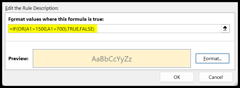
- In the end, click OK to apply the rule.
Now you have all the cells with values below 700 or above 1500 highlighted.
A conditional formatting formula only needs to return TRUE or FALSE, so you don’t need the IF part. This shorter formula does the same job:
=OR(A1>1500,A1<700)
And if you want to highlight the values between 700 and 1500 instead, use AND, as both conditions need to be true:
=AND(A1>=700,A1<=1500)
In both formulas, A1 is the first cell of the range you selected. Excel adjusts the reference for every other cell in the range.
Using Multiple Conditions with Multiple Columns
If you want to highlight cells by applying multiple conditions to two different columns, you can do that.
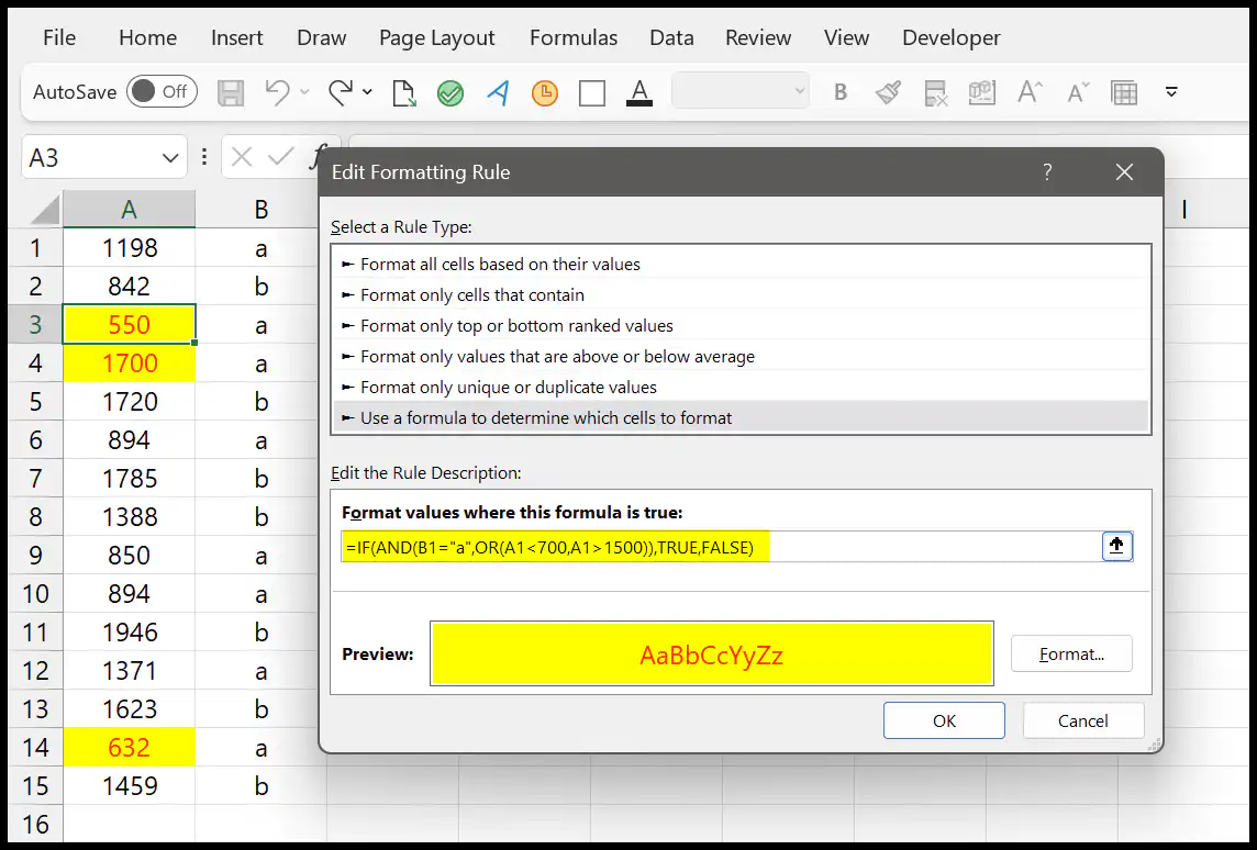
=IF(AND(B1="a",OR(A1<700,A1>1500)),TRUE,FALSE)
In the above conditional formatting, we have used three conditions to test:
- In column B, it needs to be the value “a”.
- And in column A, the value needs to be below 700 or above 1500.
That means it will test one condition first from column B, then go to column A and test two more conditions there to highlight cells.
If you select both columns (or the whole table) to highlight the entire row, add a $ before the column letters, so every cell in the row checks columns A and B:
=AND($B1="a",OR($A1<700,$A1>1500))
Without the $, a cell in column B would check column C and column B instead, and the highlight would go to the wrong cells.
Frequently Asked Questions
How many conditional formatting rules can I apply to one range?
There’s no small limit in current Excel versions, so you can add as many rules as you need. But many rules on large ranges can slow the workbook down, so combine conditions in one formula where you can.
Why is only one of my two rules showing?
Both rules may be true for the same cell, and the higher rule’s fill color covers the lower one. Check the order in Manage Rules, and check whether Stop If True is ticked.
Can I use a cell value in the condition instead of a number?
Yes. Lock the cell with $, like =OR(A1>$E$1,A1<$E$2), and then you can change the limits in E1 and E2 without editing the rule.

Written by
Puneet Gogia
Microsoft MVP — Excel · Founder, Excel Champs
Twelve years of teaching Excel, and a decade before that using it as a data analyst. Every tutorial here is written from a file I actually built.