Conditional formatting can be applied based on another cell only when you use a custom formula rule.
Instead of letting Excel check the selected cell itself, you write a formula that points to a different cell, and whenever that formula returns TRUE, Excel applies the formatting. If it returns FALSE, nothing happens.
This gives you full control to highlight rows, columns, or ranges based on any cell in your spreadsheet.
Have you ever wanted Excel to highlight an entire row when a specific cell meets a condition? Or maybe you want cells to change color based on what someone selects from a dropdown? If yes, I have something for you.
The problem is that, by default, conditional formatting only looks at the cell you are applying it to. It does not look at another cell. And that leaves a lot of people stuck.
But here is the good news. With a small trick, using a custom formula inside the conditional formatting rule, you can make Excel look at any cell you want. It is surprisingly simple once you see it in action.
I have been working with Excel for over 10 years, and conditional formatting based on another cell is one of those features I use almost every single week. Let me walk you through all five methods, step by step.
How Conditional Formatting Based on Another Cell Works
Before we jump into the methods, let me quickly explain how this actually works. It will make every step below much easier to follow.
Normally, when you apply conditional formatting, Excel checks the value of the cell you selected. For example, if cell A1 is greater than 100, highlight A1. Simple. But the problem is, the cell being checked and the cell being highlighted are always the same.
 Default Behavior
Excel checks the selected cell and highlights that same cell. You cannot point it to a different cell by default.
 What We Want
Excel checks another cell — say, a status column — and highlights a completely different range, like an entire row.
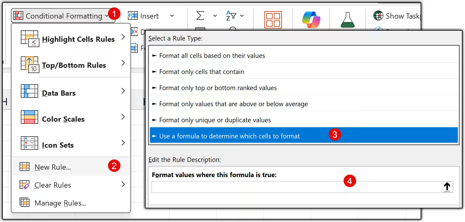
The trick is to use the "Use a formula to determine which cells to format" option inside the conditional formatting rules. This option lets you write any formula you want, and that formula can point to any cell in your spreadsheet.
 Key Idea
When you use a formula-based rule, the formula returns either TRUE or FALSE. If it returns TRUE, Excel applies the formatting. If it returns FALSE, nothing happens. That is all there is to it.
Key Idea
When you use a formula-based rule, the formula returns either TRUE or FALSE. If it returns TRUE, Excel applies the formatting. If it returns FALSE, nothing happens. That is all there is to it.
Now, there is one thing that you need to take care of, and that is cell references. Whether you lock the column, the row, or both with a $ sign makes a huge difference in how the formatting spreads across your range. But do not worry, I will call this out clearly in each method below.
Alright, let's get into it.
Method 1: Highlight a Row Based on a Single Cell Value
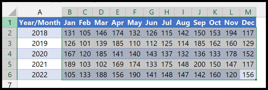
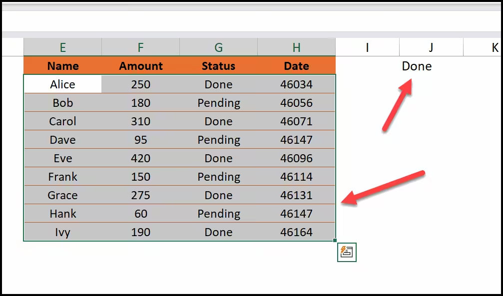
Let's start with the most common scenario. You have a data table and you want Excel to highlight rows whenever the values in a column are greater than or equal to a number you type in a reference cell. The moment you change that number, the highlighting updates automatically.
In this example, cell O1 is our reference cell. Whenever a value in column B is greater than or equal to whatever is in O1, Excel will highlight that row. Here are the steps to set this up.
-
First, select the range where you have your data. Make sure you select the full range — all the columns you want to highlight, excluding the header row.
-
After that, go to the Home tab, click on Conditional Formatting, and then click New Rule.
Home Tab ➜ Conditional Formatting ➜ New Rule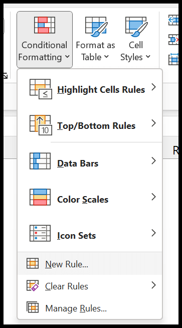
-
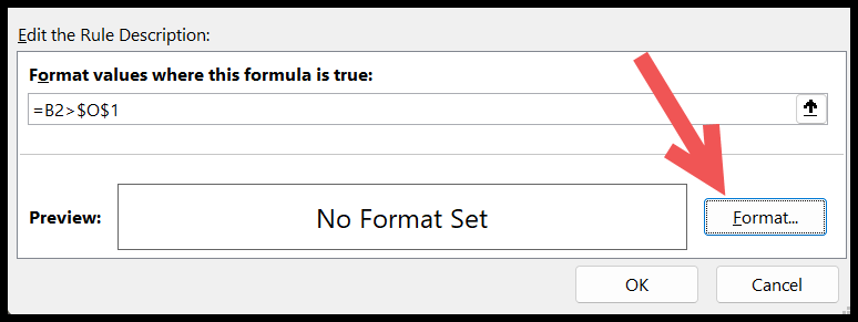
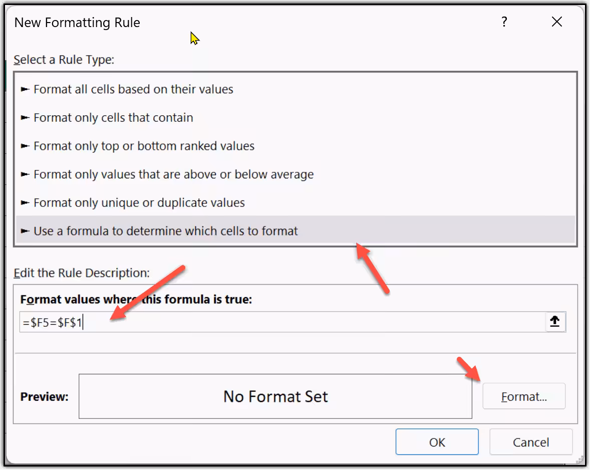
In the New Rule dialog box, click on "Use a formula to determine which cells to format." Then, in the formula input bar, type in the following formula.
=B2>=$O$1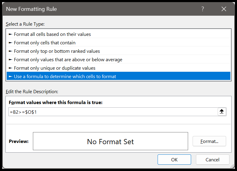
-
Next, click the Format button to choose the format you want to apply — pick a fill color, a font color, or both. As you can see, a preview will show you exactly how it will look.
-
In the end, click OK to apply the rule, and then click OK again to close the Rules Manager. That is all.
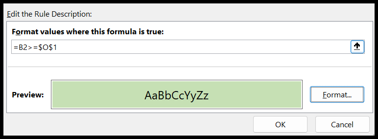
As you can see, the rows where column B values are greater than or equal to the number in cell O1 are now highlighted. The best part? The moment you change the value in O1, the formatting updates instantly, no need to touch the rule at all.
How This Formula Works
Let me quickly break down what each part of that formula is doing.
- B2 This points to the first cell in the column you want to check. The column is left unlocked so it can shift across columns, and the row is left free so it moves down row by row.
- >= The "greater than or equal to" operator. The formula returns TRUE whenever the value in B2 is equal to or above the threshold.
- $O$1 This is the reference cell that holds your threshold number. Both the column and row are locked with $ signs so Excel always looks at exactly cell O1 — no matter which row or column it is evaluating.
 One thing to take care of: Notice that B2 has no dollar signs, but $O$1 has both. This is intentional. B2 needs to shift as Excel checks each row. O1 must stay fixed because it is your threshold cell. Mix these up and the formatting will not work correctly.
Method 2: Highlight Cells Based on Another Cell's Text Value
Now let's say you do not want to match an exact word, instead, you want Excel to highlight rows whenever a cell contains a specific text.
For example, highlight every row where the category column contains the word "Marketing," even if the full text says "Digital Marketing" or "Marketing Team."
This is where the SEARCH function comes in. Unlike a direct equals check, SEARCH looks for your text anywhere inside the cell, partial matches included. Here are the steps to do this.
-
First, select the full data range where you want to apply the formatting. Make sure you start from the first data row and exclude the header.
-
After that, go to the Home tab, click on Conditional Formatting, and then select New Rule.
Home Tab ➜ Conditional Formatting ➜ New Rule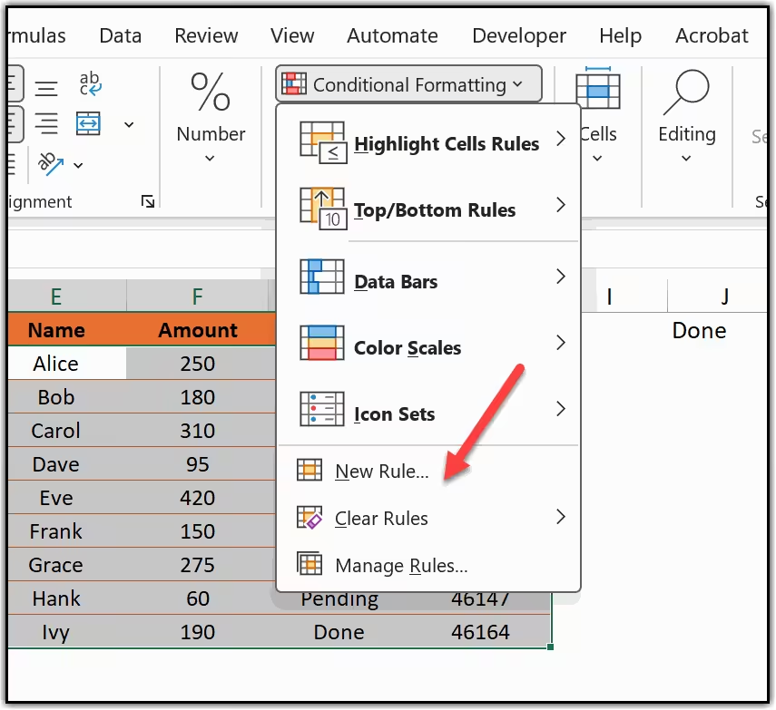
-
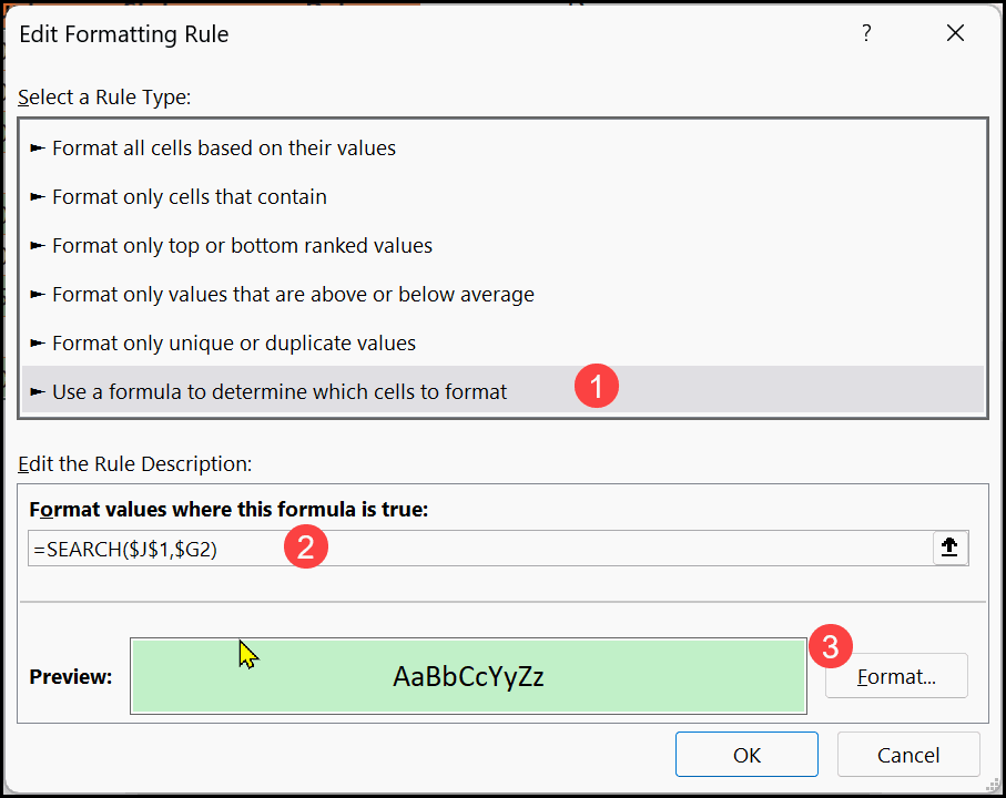
In the New Rule dialog box, click on "Use a formula to determine which cells to format." Then, in the formula bar, enter the following formula.
=SEARCH($G$1,$B2)Here, G1 is the cell where you will type the text you want to search for, and B is the column being checked.
-
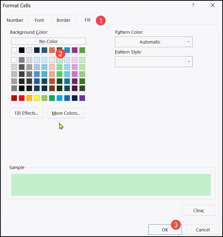
Next, click the Format button and choose the fill color or font style you want to apply when the text is found. Click OK once you are done.
-
In the end, click OK to apply the rule and then OK again to close the Rules Manager. That is all.
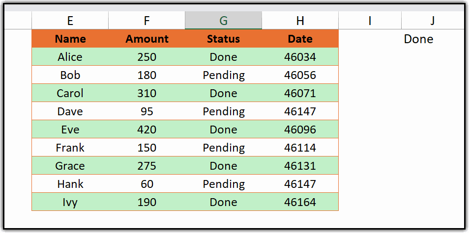
As you can see, all the rows where column B contains the text you typed in cell G1 are now highlighted. And here is the moment of joy — the moment you type a different word in G1, the highlighting updates across the entire sheet instantly.
Method 3: Highlight a Row When a Cell is Blank or Not Blank
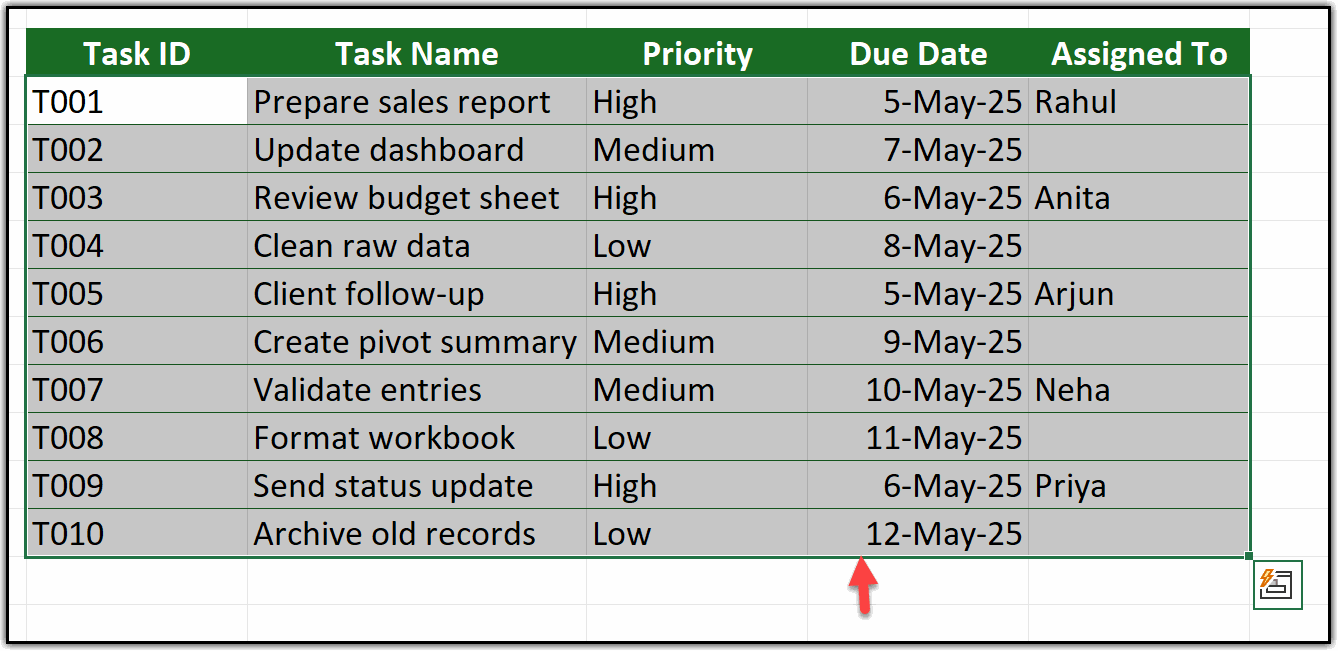
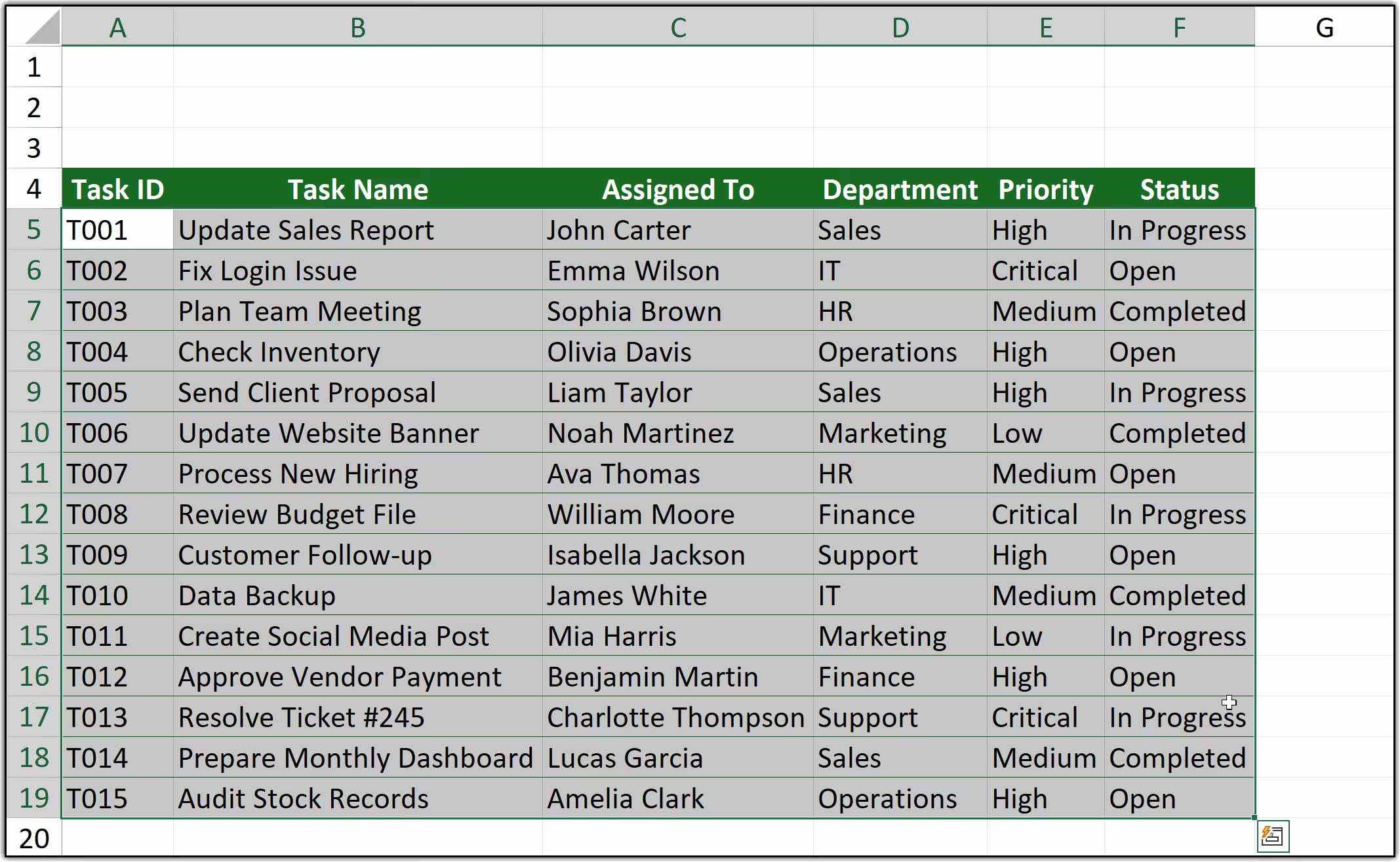
Here is a scenario I come across a lot. You have a list of tasks or records, and some rows are missing a value in an important column — say, the Assigned To column. You want to visually flag every row where that cell is empty so nothing slips through the cracks.
For this, we use the ISBLANK function inside the conditional formatting rule. And the good news is — the same setup works for highlighting rows that are not blank too. Just one small change in the formula. Let me walk you through it.
-
First, select the full data range where you want to apply the formatting. Start from the first data row and include all the columns you want to highlight.
-
After that, go to the Home tab, click on Conditional Formatting, and then click New Rule.
Home Tab ➜ Conditional Formatting ➜ New Rule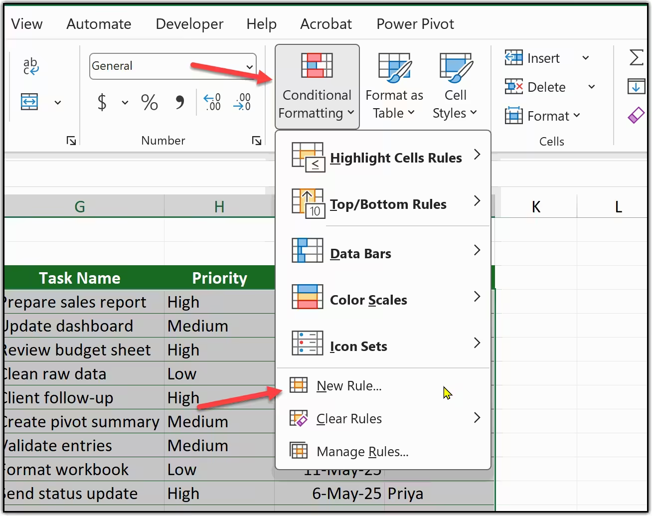
-
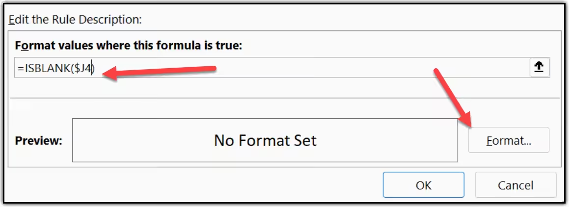
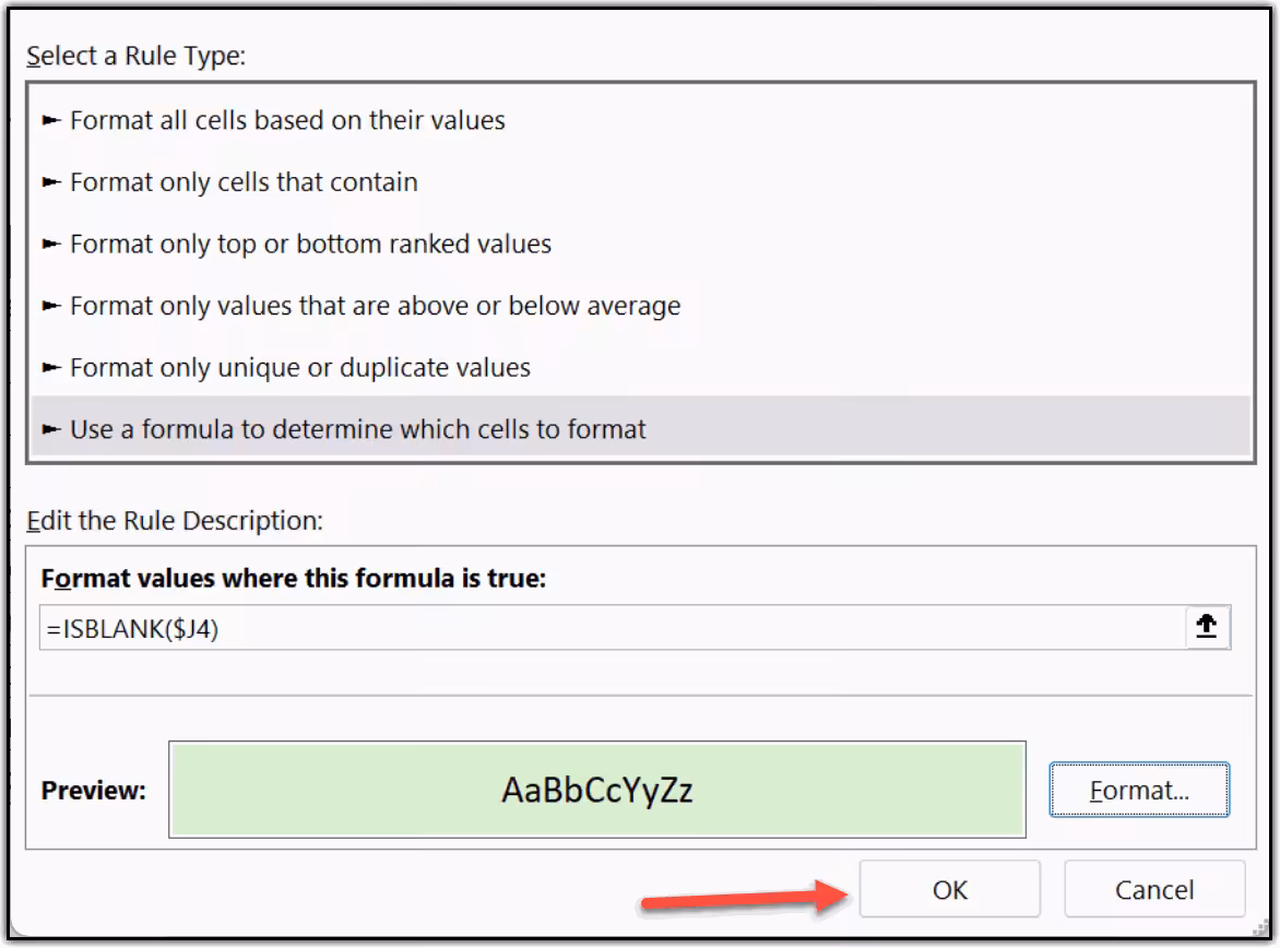
In the New Rule dialog box, select "Use a formula to determine which cells to format." Now, depending on what you want to highlight, enter one of these two formulas in the formula bar.
Blank
=ISBLANK($C2)Highlights rows where column C is empty
Not blank
=NOT(ISBLANK($C2))Highlights rows where column C has a value
-
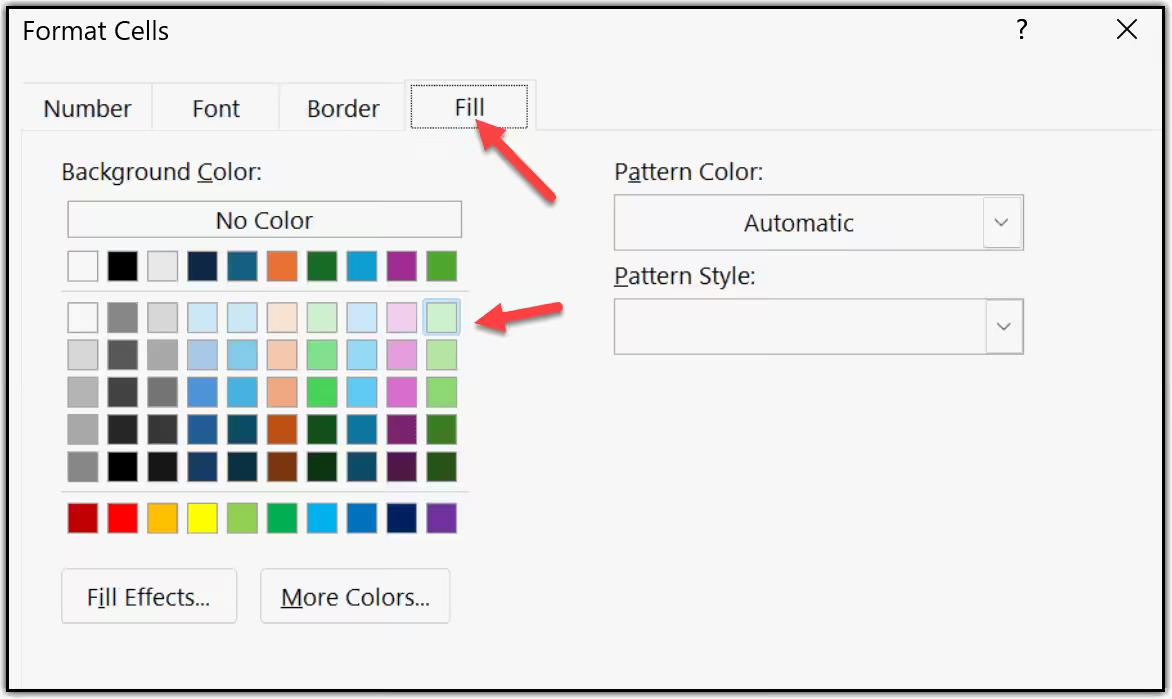
Next, click the Format button and pick your fill color. A light red or orange works well for blank rows since it signals something is missing. Click OK once you are happy with the format.
-
In the end, click OK to apply the rule and then OK again to close the Rules Manager. That is all.
As you can see, every row where the Assigned To column is empty is now highlighted. The moment someone fills in that cell, the highlight disappears automatically — no manual work needed.
Method 4: Highlight Based on a Drop-Down List Value (Dynamic)
This one is my personal favorite. Instead of hardcoding a value into your formula, you connect the conditional formatting rule to a drop-down list. So whenever someone picks a different option from the dropdown, the entire highlighting updates automatically — no editing rules, no touching formulas.
In my experience, this is incredibly useful for dashboards and trackers where the viewer needs to quickly filter and highlight different categories on the fly. Let me walk you through how to set this up.
Part A — Create the Drop-Down List
-
First, click on the cell where you want to place the drop-down list. This will be your control cell — let's say F1. After that, go to the Data tab and click on Data Validation.
Data Tab ➜ Data Tools ➜ Data Validation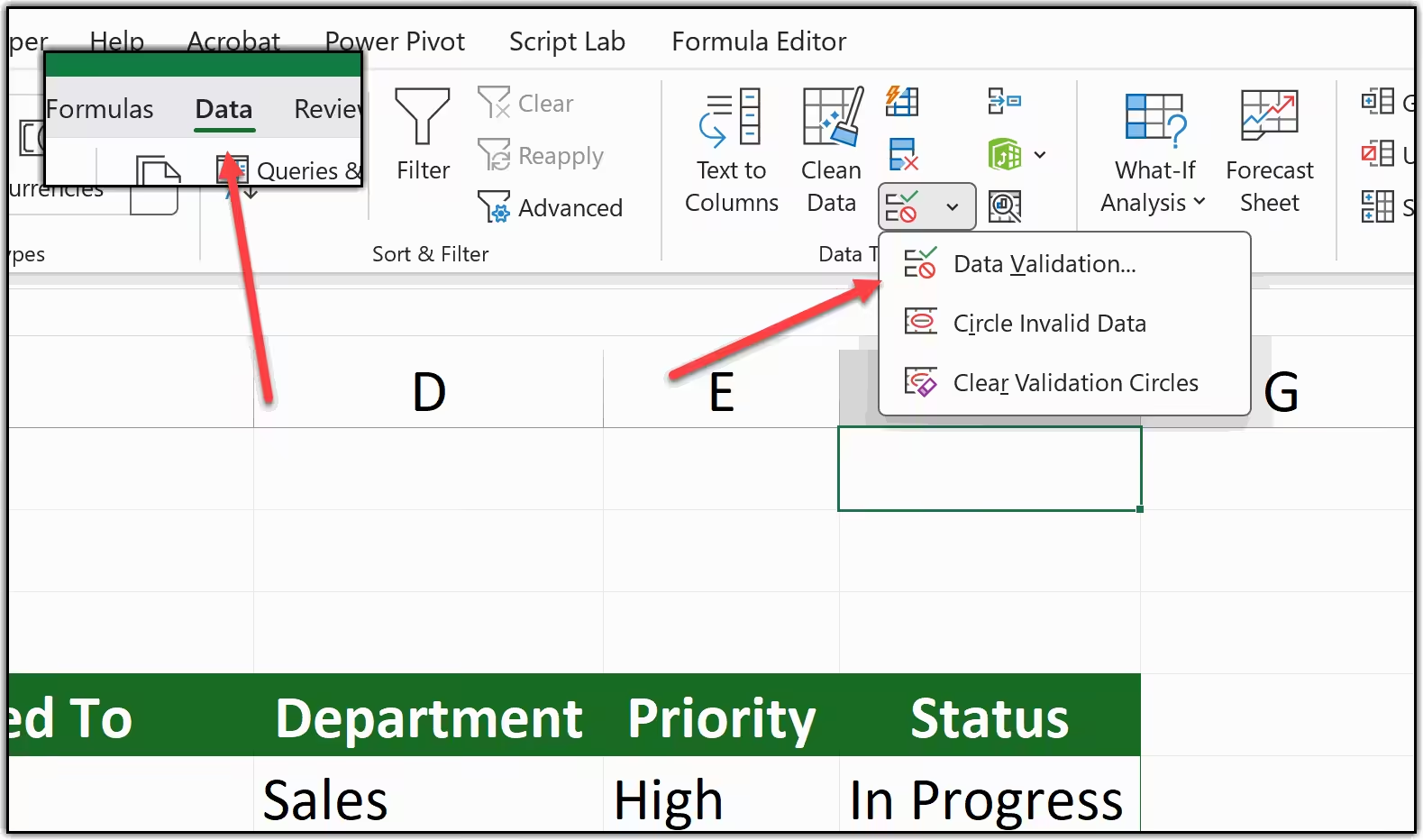
-
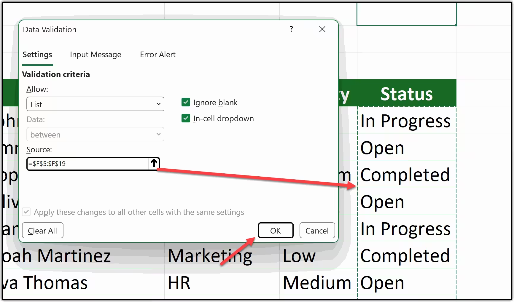
In the Data Validation dialog box, under the Allow dropdown, select List. Then in the Source field, type in your options separated by commas — for example, Pending, In Progress, Done. Click OK.
-
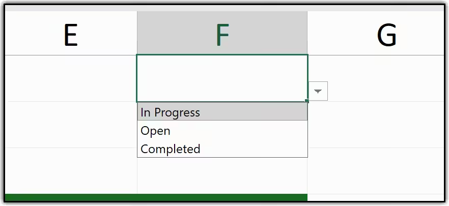
As you can see, cell F1 now has a drop-down arrow. You can click it and pick any of the options you added. Now let's connect this to the conditional formatting rule.
Part B — Connect the Drop-Down to Conditional Formatting
-
First, select the full data range that you want to highlight — for example, A2:D10.
-
After that, go to Conditional Formatting and click New Rule.
Home Tab ➜ Conditional Formatting ➜ New Rule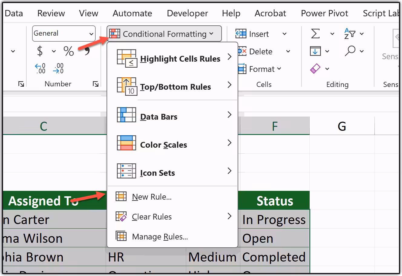
-
Select "Use a formula to determine which cells to format" and enter the following formula in the formula bar:
=$D2=$F$1Where D is your Status column and F1 is the drop-down cell.
Next, click the Format button, choose your highlight color, and click OK.
-
In the end, click OK to apply the rule and OK again to close the Rules Manager. That is all.
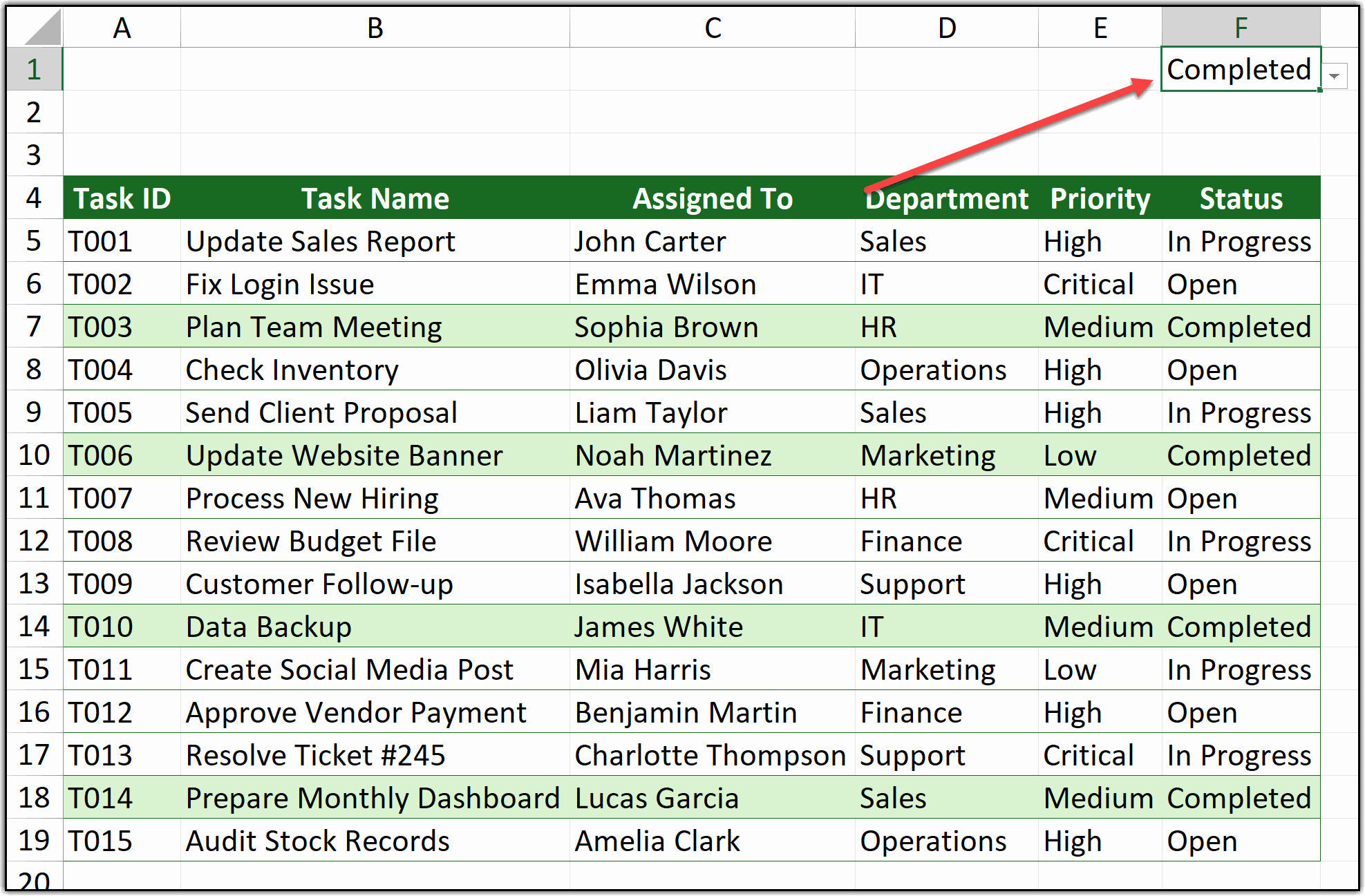
Now go ahead and click the drop-down in F1. The moment you pick a different option — say "In Progress" — Excel will instantly highlight every row where the Status column matches that value. And the moment of joy? Change it again and watch the whole sheet update in real time.
Method 5: Highlight Based on a Date in Another Cell
This last method is one that I find extremely useful for project trackers and deadline sheets. The idea is simple, you want Excel to highlight rows based on dates.
For example, highlight every task that is overdue, or highlight rows where the due date is within the next 7 days, or flag anything due today.
For all of this, we combine the power of conditional formatting with Excel's TODAY() function. Since TODAY() always returns the current date, your highlighting updates automatically every single day, without you touching anything.
-
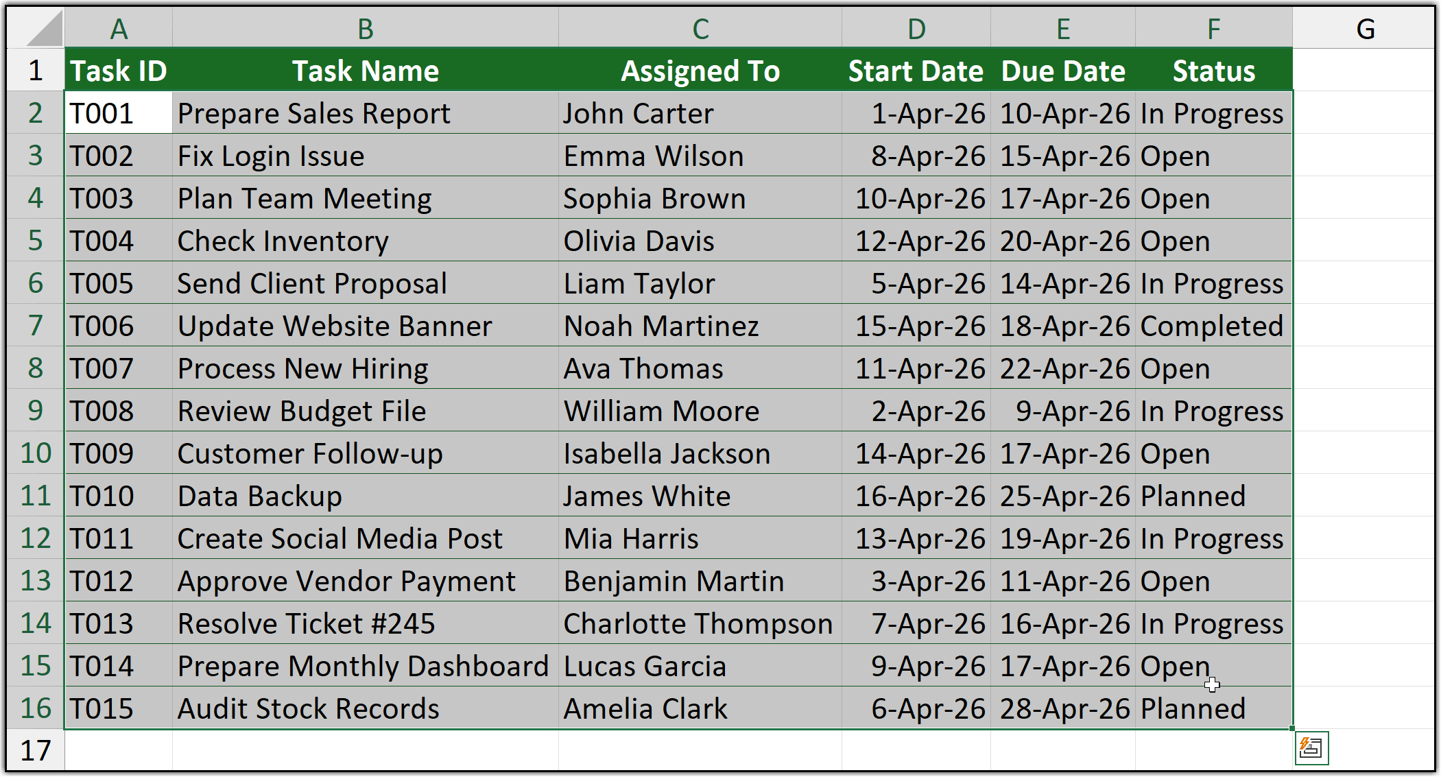
First, select the full data range where you want to apply the formatting. In this example, select A2:D10 — your full table excluding the header row.
-
After that, go to the Home tab, click on Conditional Formatting, and then click New Rule.
Home Tab ➜ Conditional Formatting ➜ New Rule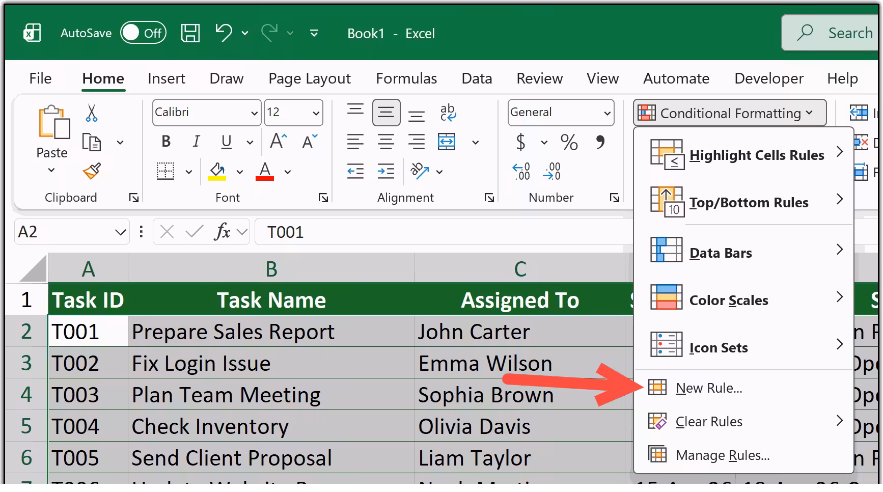
-
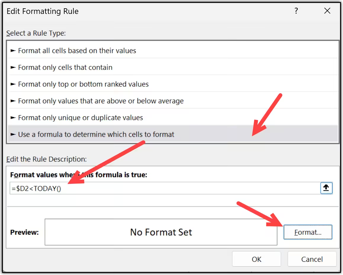
In the New Rule dialog box, select "Use a formula to determine which cells to format." Now, depending on what you want to highlight, pick one of these formulas and enter it in the formula bar.
Overdue
=$C2<TODAY()Due date has passed
Due today
=$C2=TODAY()Due date is today
Next 7 days
=$C2<=TODAY()+7Due within a week
-
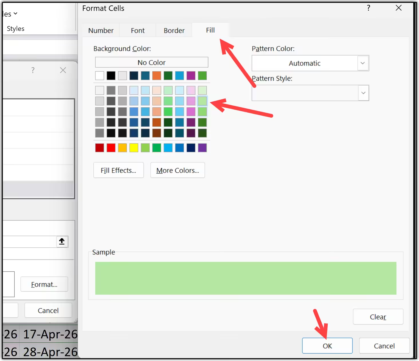
Next, click the Format button and choose your color. A red fill works well for overdue rows, yellow for due today, and orange for upcoming deadlines. Click OK once you are done.
-
In the end, click OK to apply the rule and OK again to close the Rules Manager. That is all.
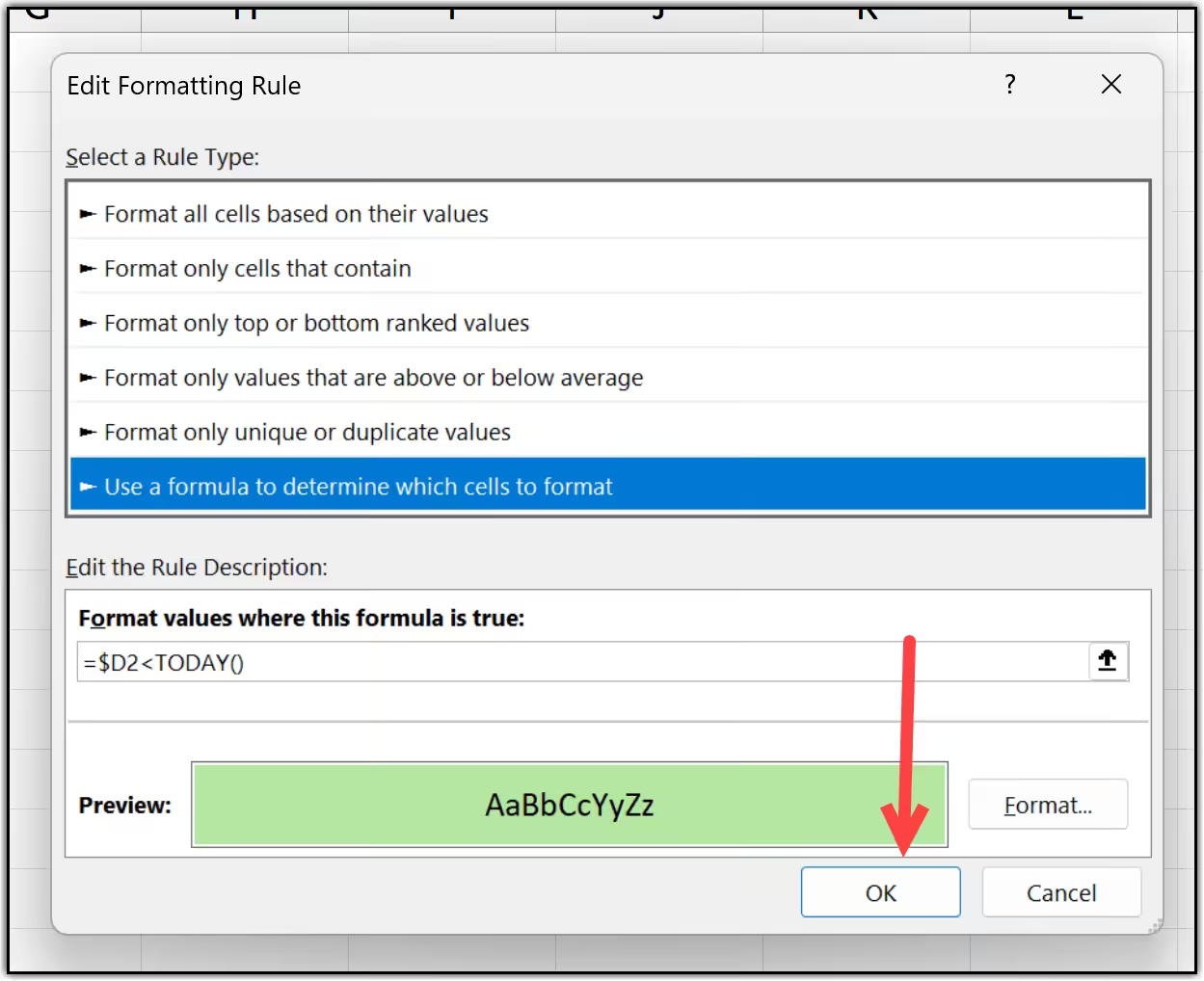
As you can see, the rows are now highlighted based on their due dates. And here is the best part — since the formula uses TODAY(), every time you open this file, Excel recalculates the dates and updates the highlighting automatically. You never have to touch the rule again.
Important Things to Keep in Mind
Before you go ahead and apply these methods to your own data, there are a few things I want to flag. In my experience, these are the points where most people run into trouble, and knowing them upfront will save you a lot of head-scratching later.

Absolute vs Relative Cell References: This is the Big One
This is the one key thing you need to remember across every method in this tutorial. The $ sign in your formula controls whether Excel locks a reference or lets it shift as the rule is applied across your range. Here is a quick reference so you always know which one to use.
Reference | What it does | When to use it |
|---|---|---|
$D$2 |
Locks both column and row — always points to exactly D2 |
For a single fixed cell like a threshold or dropdown (e.g. $O$1, $F$1) |
$D2 |
Locks the column, row shifts freely down the range |
For checking a specific column across all rows — most common in row-highlighting rules |
D$2 |
Locks the row, column shifts freely across the range |
Rarely used in conditional formatting — mostly for column-by-column comparisons |
D2 |
No lock — both column and row shift freely |
Almost never used in conditional formatting rules |

Always Select the Right Range Before Creating the Rule
The range you select before opening Conditional Formatting determines where the rule gets applied. If you want to highlight full rows, select all the columns in your table, not just one column. And always exclude the header row from your selection, otherwise your header might get highlighted too.

Rule Priority Matters When You Have Multiple Rules
If you apply more than one conditional formatting rule to the same range, Excel applies them in priority order, the rule at the top of the list wins. You can manage this by going to Conditional Formatting ➜ Manage Rules and using the up and down arrows to reorder them. If two rules conflict on the same cell, only the top rule's format will show.

Formula-Based Rules Do Not Update Automatically on Every Keystroke
Excel recalculates conditional formatting rules when you make a change to the sheet or press F9 to force a recalculation. In most cases this is instant and you will not notice any delay. However, on very large datasets with many rules, you might see a slight lag. If that happens, try reducing the number of rules or narrowing the applied range.
In the End
These are the five methods you can use to apply conditional formatting based on another cell in Excel. Let me do a quick recap of everything we covered.
All five methods use the same core idea, a formula-based conditional formatting rule that points to another cell.
Once you understand that concept, you can mix and match these approaches to build some really powerful, dynamic spreadsheets.
I must say, the drop-down method is my personal favorite because it turns a static spreadsheet into something that feels almost interactive.
But every method here has its place depending on what your data looks like and what you are trying to highlight.
Frequently Asked Questions
Here are the answers to some common questions I get about conditional formatting based on another cell. If you are stuck on something not covered here, drop your question in the comments below and I will help you out.
Yes, you can — but only in the desktop version of Excel. In the formula-based rule, reference the other sheet using the syntax =Sheet2!$A$1>100. If your sheet name contains spaces, enclose it in single quotes, like ='Sales Data'!$A$1>100.
In some older versions of Excel (2010 and earlier), cross-sheet references in conditional formatting formulas can be unreliable. If you run into issues, a workaround is to create a Named Range that points to the cell on the other sheet, and then use that name in your formula instead.
This is the most common issue people run into, and it is almost always caused by one of these three things:
1. Wrong cell references. The reference cell (like $O$1) must be locked with dollar signs so it stays fixed.
2. The "Applies to" range is wrong. Open Conditional Formatting → Manage Rules and check the range shown.
3. The formula is returning an error. If your formula produces an error (like #VALUE! or #N/A), Excel treats it as FALSE.
If the sheet still does not update, press Ctrl + Alt + F9 to force a full recalculation.
Yes. Wrap your conditions inside AND() or OR() depending on what you need:
Both conditions must be true: =AND($B2>=$O$1,$D2="Done")
At least one condition must be true: =OR($B2>=$O$1,$D2="Done")
See my tutorial on multiple conditions in conditional formatting.
Excel for the web: Supports basic conditional formatting rules but formula-based options may be limited.
Google Sheets: Yes, the same approach works using Custom formula is.
There is no hard limit, but I recommend keeping it under 10 rules per range.
Check Conditional Formatting → Manage Rules → This Workbook to clean extra rules.
SEARCH is not case-sensitive and supports wildcards.
FIND is case-sensitive and does not support wildcards.
It can if you apply too many rules on large ranges.
Avoid volatile functions like TODAY(), NOW(), INDIRECT() on wide ranges.
Yes. Example:
=NOT(ISNA(VLOOKUP($A2,LookupTable!$A:$B,1,FALSE)))

Which method worked best for you?
I would love to hear from you. Please share your views with me in the comment section below — which one of these five methods did you end up using, and was there a scenario it solved that you had been stuck on for a while? I'd love to hear from you.