

Select both columns starting at the first data row, for example A2:B100, then go to Home → Conditional Formatting → New Rule → Use a formula to determine which cells to format. Enter =$A2<>$B2, click Format, pick a fill and click OK twice. Every row where the two values differ is highlighted in both columns.
To highlight the rows that match instead, use =$A2=$B2. The $ before each column letter locks the rule to columns A and B, while the unlocked row number lets it move down one row at a time.
To check whether a value appears anywhere in the other column, not only on the same row, select A2:A100 and use =COUNTIF($B$2:$B$100,A2)>0. Change >0 to =0 to highlight the values missing from column B.
For a check with no formula, select both columns and go to Home → Conditional Formatting → Highlight Cells Rules → Duplicate Values, then choose Duplicate or Unique. This treats both columns as one list, so a value repeated inside column A alone is highlighted too. Use the COUNTIF rule when you need a strict column-to-column match.
The comparison ignores case, so apple and Apple count as equal; use =NOT(EXACT($A2,$B2)) when case matters. If values that look identical still show as different, look for trailing spaces or numbers stored as text in one column. And keep the row in the formula equal to the first selected row: select from row 1 but type $A2, and every highlight lands one row out.
In Excel, conditional formatting is the easiest way to compare two columns. With this, you can compare two columns in multiple ways. In this tutorial, we will learn multiple methods to use conditional formatting for column comparison.
Compare Two Columns Row-Wise
With this method, you can compare both cells from each row of the columns and highlight the cells with the same value.
- First, select both columns in the data.

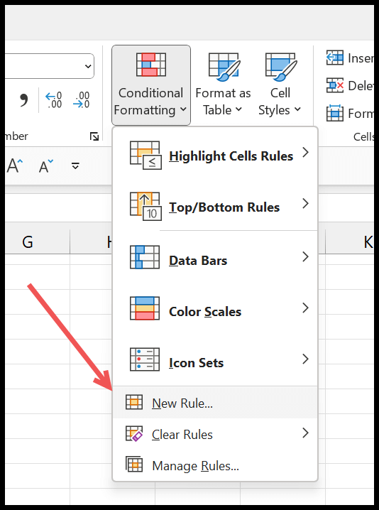
- Afterward, go to the Home Tab > Conditional Formatting > New Rule.
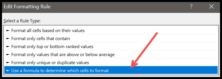
- From there, click on “Use a formula to determine which cells to format”.
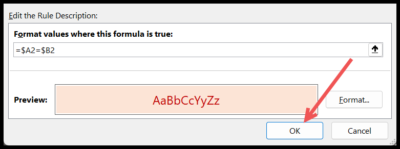
- Next, in the formula box, enter the formula =$A2=$B2, then click “Format…” to specify the format.

- Once you specify the format, click OK to apply the conditional formatting and again OK to close the Rules Manager.
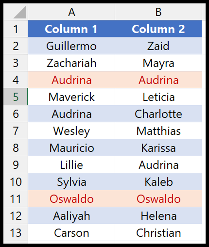
And the moment you click OK, it highlights cells from both columns where values are the same.
Here’s the formula you need for this rule. The $ before the column letters locks the columns, so every cell in the row looks at columns A and B, while the row number (2, the first row of the selection) changes from row to row:
=$A2=$B2
And if you want to highlight the rows where the values are different, use the following formula instead:
=$A2<>$B2
This comparison isn’t case-sensitive, so “Apple” and “apple” count as the same. To compare with the case as well, use EXACT. The following formula highlights the rows where the values differ, even only in case:
=NOT(EXACT($A2,$B2))
Compare All the Values from All the Columns
Unlike the first method, here you can highlight values that are duplicates across both columns, no matter which row they are in. And for this, select both columns and go to the Home Tab > Conditional Formatting > Highlight Cells Rules > Duplicate Values.
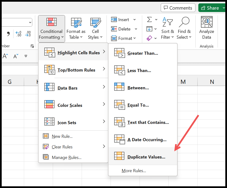
In the duplicate values dialog box, select which values you want to highlight and the color you want to apply.
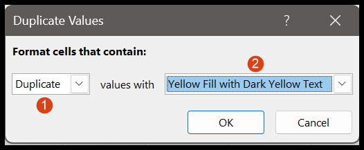
In the end, click OK to apply the conditional formatting.

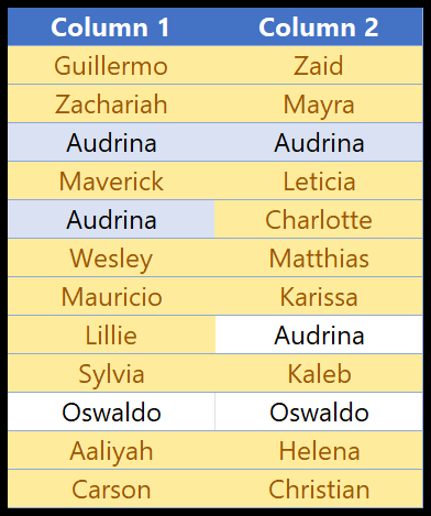
The moment you click OK, all the cells where values are duplicate in both columns will be highlighted with the format you have selected. But if you want to highlight the cells which are unique in both columns, you need to select “Unique” from the drop-down.
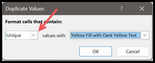
And when you click OK, it will highlight the values that appear only once across both columns.
Keep in mind that Duplicate Values also highlights a value that appears twice in the same column, even if it isn’t in the other column at all.
Highlight Values Missing from the Other Column
To find the values in column A that aren’t anywhere in column B, select the values in column A (like A2:A10), create a new rule with “Use a formula to determine which cells to format”, and use the following formula. COUNTIF counts how many times the value appears in column B, and the rule formats the cell when the count is 0:
=COUNTIF($B$2:$B$10,$A2)=0
And to do the same for column B, select B2:B10 and swap the columns in the formula:
=COUNTIF($A$2:$A$10,$B2)=0
Highlight the Entire Row
The row-wise formula also works when you select the whole table (like A2:D10) instead of only the two columns. As the columns are locked with $, each cell checks columns A and B of its own row, so the whole row gets highlighted.
Frequently Asked Questions
Why are matching values not highlighted?
Usually, one of the values has an extra space, or one is a number and the other is a number stored as text (5 and “5” aren’t equal). Use TRIM to clean the spaces and convert the text numbers to real numbers.
Why does the rule highlight the wrong rows?
The row number in the formula must be the first row of your selection. If you select from row 2, use $A2; if you select from row 1, use $A1. Also, don’t put a $ before the row number.
Can I compare two columns on different sheets?
Yes. In current versions of Excel, the formula can refer to another sheet, like =$A2=Sheet2!$A2. In very old versions (Excel 2007 and earlier), you need a named range for the other sheet.

Written by
Puneet Gogia
Microsoft MVP — Excel · Founder, Excel Champs
Twelve years of teaching Excel, and a decade before that using it as a data analyst. Every tutorial here is written from a file I actually built.