

INDIRECT turns a text string into a real cell reference, which lets one VLOOKUP pull from several sheets. Put the sheet names in a header row, then build the reference from them: =VLOOKUP($A2,INDIRECT("'"&B$1&"'!A:B"),2,0).
If B1 contains “Jan”, INDIRECT converts ‘Jan’!A:B into a live reference to that sheet, and dragging the formula across to the Feb column switches the sheet automatically. The single quotes matter — they’re what makes sheet names containing spaces work, so keep them even when your names are simple.
Two things to watch. If the sheet name in the header doesn’t exactly match a real tab, INDIRECT returns #REF! with no hint about which part is wrong, so check for trailing spaces first.
And INDIRECT can’t read a closed workbook at all — it only works on sheets in an open file. It’s also volatile, meaning it recalculates on every change in the workbook, so on a large grid of these formulas you’ll notice the slowdown.
If you want to use VLOOKUP and the data you want to look up is in different sheets, you can combine it with the INDIRECT. It helps you to define multiple ranges in a single formula.

In the above example, we have month-wise data in three different worksheets. But with a single VLOOKUP + INDIRECT, you can get quantity for all the products from all the months from multiple sheets.
=VLOOKUP($A2,INDIRECT("'"&B$1&"'!"&"A:B"),2,FALSE)To understand this formula, you need to split it into two parts:
In the first part, we have the INDIRECT function, which creates a reference to the sheet by using the name from row 1. In the example below, we reference the sheet Jan’s range A:B.
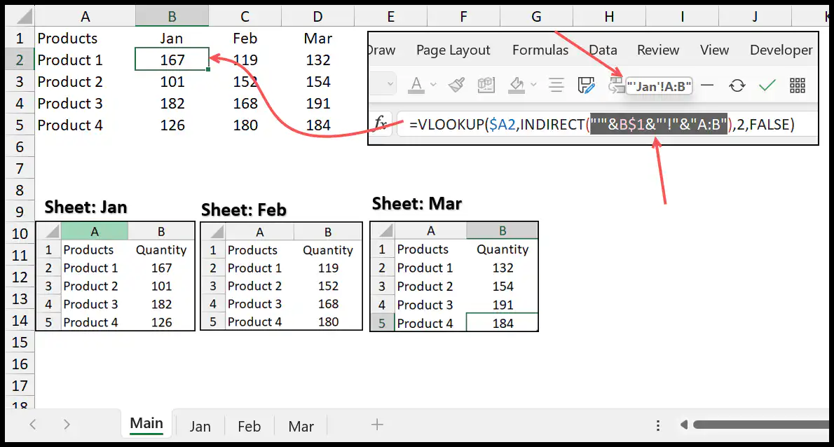
You need to create a structure within the INDIRECT to reference the sheet with the name and the range where you have the data.
=INDIRECT("'"&B$1&"'!"&"A:B")Once you move the formula to the Feb column, the reference in the INDIRECT changes to the sheet Feb.
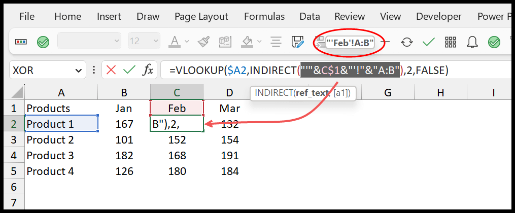
In the second part, VLOOKUP uses the table range address returned by the INDIRECT and gets its values according to the col_index_num specified in the range.
Important Point
In the above formula, you need the right structure to reference a range with the sheet name. If you enter the below structure in the INDIRECT:
"'"&B$1&"'!"&"A:B"It will return:
"'Jan'!A:B"Alternative Method
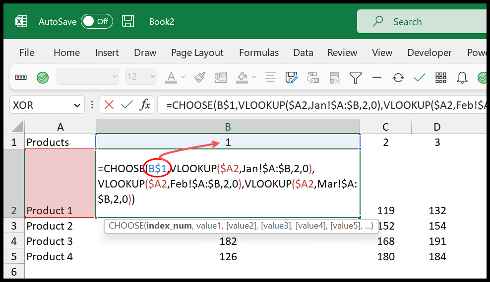
INDIRECT is a Volatile function. It updates itself when there’s any change in the worksheet. That’s why you can consider using CHOOSE. For example, with CHOOSE, you can write three formulas using VLOOKUP.
=CHOOSE(B$1,VLOOKUP($A2,Jan!$A:$B,2,0),VLOOKUP($A2,Feb!$A:$B,2,0),VLOOKUP($A2,Mar!$A:$B,2,0))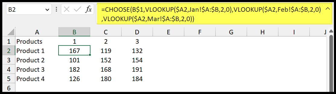
In this formula, as I said, we have three VLOOKUPs, and when with the CHOOSE, you can decide to get the result from any of the VLOOKUPs
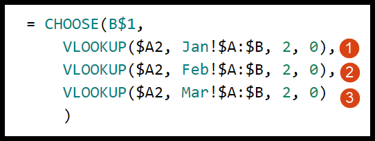
In the CHOOSE, we have referred to the B1; in Row 1, you have index numbers to use to get the formula value from the CHOOSE.
For example, when you have 2, CHOOSE will return the value for the second VLOOKUP; from the third, there are 3.
Written by
Puneet Gogia
Microsoft MVP — Excel · Founder, Excel Champs
Twelve years of teaching Excel, and a decade before that using it as a data analyst. Every tutorial here is written from a file I actually built.