

To keep row 1 visible as you scroll, go to View → Freeze Panes → Freeze Top Row, or press Alt → W → F → R. To freeze more header rows, select the cell in column A directly below the last header row (A3 for two rows) and choose View → Freeze Panes → Freeze Panes.
To make row 1 a real header row, click inside the data, press Ctrl + T, tick My table has headers and click OK. The headers get filter buttons, and when you scroll down they replace the column letters at the top of the sheet, so you don’t need to freeze anything.
To repeat row 1 on every printed page, go to Page Layout → Print Titles and enter $1:$1 in Rows to repeat at top. In Power Query, use Home → Use First Row as Headers when imported data comes in with generic Column1, Column2 names.
If Freeze Panes is greyed out, you’re in Page Layout view or still editing a cell. Press Esc and switch to View → Normal. The column letters A, B, C themselves can’t be renamed.
Headers are a very important part of data structure, making the data easier to read and understand. They help users understand what kind of data the cells under different columns will have, based on the header names.
So, everyone who works in Excel knows the importance of having the first row of your data set as a header row.
Let’s take an example: Let’s say you have sales data with names, dates, and amounts. With headers, it’s easier to tell which column is which. To keep the header row in view, click “View” > “Freeze Panes” > “Freeze Top Row” to keep the top row visible.
This way, you see the column titles even when you scroll down. This makes your data clear and easy to understand.
This tutorial will explain how to make the first row of your data a header row in four different ways, including the one I have mentioned above.
- Method 1: You can use the Freeze Panes option. Go to View > Freeze Panes > Freeze Top Row.
- Method 2: Convert data into an Excel Table. Go to Home > Format as Table or use the keyboard shortcut Ctrl + T.
- Method 3: To use Power Query, go to the Data tab > From Table/Range, and in the Power Query Editor, go to Home (or Transform) > Use First Row as Headers.
- Method 4: You can use print titles to make the first row a header in the printouts, and for this, go to Page Layout > Print Titles > “Rows to repeat at top”.
Steps to Make First Row a Header Row using Freeze Option
By applying Freeze to the first row of the data set, the first row will get frozen as the header row, and when you scroll down in the spreadsheet, the header row stays visible all the time.

- First, open the data in the spreadsheet, where you want to freeze the first row as the headers row.
- After that, go to the “View” tab and click on the “Freeze Panes” icon and then click on the “Freeze Top Row” option from the drop-down menu.
- Or use the keyboard shortcut “Alt → W → F → R” in sequence to directly choose the “Freeze Top Row” option.
- At this moment, your first row is frozen as the header row, and when you scroll down the Excel sheet, the headers stay visible all the time.
With the Freeze Panes option, you can also make more than one row a header. For this, select the cell below the last row you want to freeze (A3 for the first two rows, or A4 for the first three rows), and then click on View > Freeze Panes > “Freeze Panes”. Excel freezes all the rows above the selected cell, and you will get them at the top while scrolling. To undo it, go to View > Freeze Panes > Unfreeze Panes.
Convert Data into Excel Table to Make the First Row as Header Row
You can convert your data set into table format and make the first row a headers row by following the below steps:
- First, go to any cell within the data and then go to the “Home” tab.
- After that, click on the “Format as Table” icon and choose the table format design.
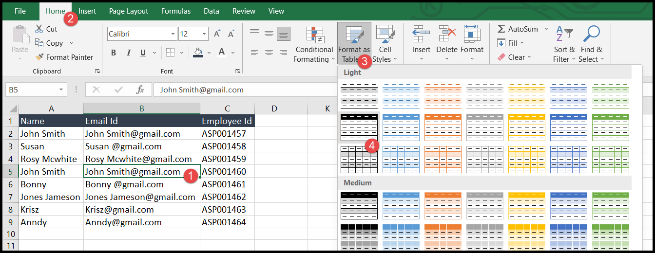
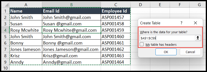
- Once you choose the table format (or press the keyboard shortcut “Ctrl + T”), the “Create Table” dialog box opens.
- Now, you will see your data range is selected automatically; just make sure the “My table has headers” option is checked and click OK.

- At this moment, the data is converted into a table with the first row as the header row, with filter buttons. When you scroll down inside the table, the table’s headers replace the column letters (A, B, C) at the top, so you can see them without freezing panes.
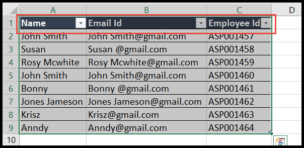
Select First Row as Header Row Using Power Query Editor
Now, let’s think about a unique problem: you have data in a workbook and want to get the data from that workbook and make the first row a header.
With Power Query, you can use the first row of values as a header. And let me tell you, loading data into Power Query and making the first row a header is easy and fun.
- First, go to any cell within the data set and go to the “Data” tab and there click on the “From Table/Range” option.

- After that, check that the selected range covers your whole data set, then uncheck the “My table has headers” option and click OK.
- Now, under the “Home” tab, click on the “Use First Row as Header” drop-down icon and then select the first option “Use First Row as Headers”.
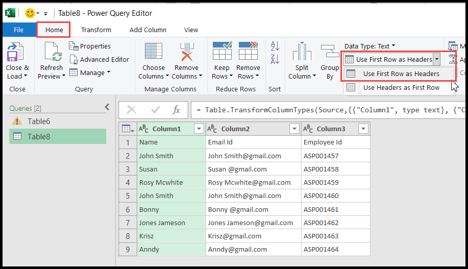
- Once you click on “Use First Row as Headers”, it will convert the first row of your data into headers.
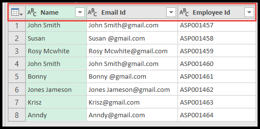
- In the end, click on the “Close & Load” icon and then click on the “Close & Load” option from the drop-down menu.
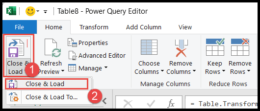
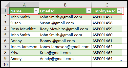
- Once you click on the “Close & Load” option, your data will be loaded to a new sheet within the same workbook, with the first row as headers.
Select First Row as Header Row using Page Layout
Many times, you need to make the first row of your data set the header row, and you want to print that header row on each page while printing the data. Follow the below steps for the same:
- First, go to the “Page Layout” tab and then click on the “Print Titles” option and it will open the “Page Setup” dialog box.

- After that, go to the “Rows to repeat at top” field and select the first header row (it shows as $1:$1), and then click on the “Print Preview” button to check if the headers are visible on all the pages.

- In the end, go to the “File” tab and click on the “Print” option or use the keyboard shortcut “Ctrl + P” to go to the “Print” dialog box to print the pages.
Which Method to Use
- Freeze Top Row: when you only want to see the headers while you scroll.
- Excel Table: when you also want filters, formatting and formulas that use the column names.
- Power Query: when the headers are in the first row of data you import, and you want them as column names.
- Print Titles: when you want the header row on every printed page.
Frequently Asked Questions
Why does Freeze Top Row freeze the wrong row?
Freeze Top Row freezes the row that is at the top of the window, not always row 1. Scroll up to the top of the sheet first (Ctrl + Home), and then apply it.
How do I turn off the header row of a table?
Select a cell in the table, go to the Table Design tab and uncheck “Header Row”. You can turn it back on from the same place.
Can I freeze the first row and the first column together?
Yes. Select cell B2 and go to View > Freeze Panes > Freeze Panes. Excel freezes row 1 and column A together.
Written by
Puneet Gogia
Microsoft MVP — Excel · Founder, Excel Champs
Twelve years of teaching Excel, and a decade before that using it as a data analyst. Every tutorial here is written from a file I actually built.