

To make negative numbers red in Excel, select your range, open Format Cells (Ctrl + 1) → Number → Custom, and enter the code 0;[Red]-0 (or 0.00;[Red]-0.00 for two decimals). Every negative value instantly turns red.
Prefer a no-code route? Use Home → Conditional Formatting → Highlight Cells Rules → Less Than, type 0, and pick a red format. All three methods only change how the number looks — the underlying value stays the same.
When you're working with a large data set or a long column of numbers, spotting the negatives at a glance is hard. Making them red fixes that in seconds — it's one of the quickest ways to make a report readable.
Below, I'll show you three fast ways to do it — Conditional Formatting, the built-in Number format, and a custom format code — plus a bonus bracket format and a VBA option. Each one takes less than a minute.
Make Negative Numbers Red Using Conditional Formatting
- Select the cells (or the range) with your numbers, go to the Home tab, and click the Conditional Formatting drop-down.
- Click Highlight Cells Rules, then choose Less Than from the list.
- In the Less Than window that opens, enter 0 in the “Format cells that are LESS THAN” box — every value below zero is a negative, so they all get caught.
- In the end, click OK, and your negative numbers turn red.


Want a different colour? Open the drop-down on the right side of the Less Than window, pick the fill you like, and click OK. That's all.

Make Negative Numbers Red Using Number Format
- Select your cells, go to the Home tab, and click the small dialog-box launcher in the corner of the Number group (or just press
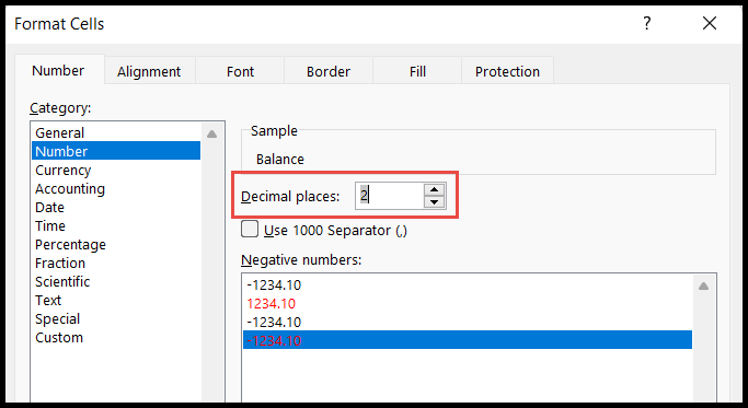
Ctrl + 1). - In the Format Cells window, open the Number tab and, under Category, select Number.
- In the Negative numbers list, choose the last option — the one that shows the number in red.
- In the end, click OK, and every negative number turns red.

By default this format adds two decimal places. If you'd rather have none (or more), use the Decimal places arrows in the Format Cells window — set it to 0 for whole numbers, or 2+ for more precision.
Make Negative Numbers Red Using Custom Format
- Select your cells, go to the Home tab, and open Format Cells (click the Number group's dialog-box launcher, or press
Ctrl + 1). - On the Number tab, choose Custom from the Category list.
- In the Type box, enter (or copy) one of the codes below, then click OK.
For whole numbers (no decimals):
0;[Red]-0Or, if you want at least two decimal places:
0.00;[Red]-0.00Here's the trick: the semicolon splits the code into two parts. The bit before it formats positive numbers and zero, and the bit after it (with [Red]) formats the negatives.

The moment you click OK, your negative numbers show up in red. That's all.

Which Method Should You Use?
All three do the same job, but each has a sweet spot. Here's how I decide:
Method | Best for | Updates live? |
|---|---|---|
Conditional Formatting | Shading the whole cell and picking from many colours | Yes |
Number Format | A fast, standard red with two decimals | Yes |
Custom Format | Full control over decimals, symbols, and brackets | Yes |
My rule of thumb: reach for Custom Format when you want the numbers themselves in red, and Conditional Formatting when you'd rather shade the entire cell.
Bonus: Show Negatives in Red with Brackets
Accountants often show losses in red and inside brackets, like (1,200). Excel has a built-in format for this: open Format Cells (Ctrl + 1) → Number → Currency (or Number), and pick the red-in-brackets option from the Negative numbers list.
Prefer a code you can reuse anywhere? Choose Custom and enter:
#,##0;[Red](#,##0)Make Negative Numbers Red Using VBA
Want a one-click, static solution? A tiny macro does it. Select your range, then run this:
' Turn negatives red, everything else black
Sub NegativesRed()
    Dim c As Range
    For Each c In Selection
        If IsNumeric(c.Value) And c.Value < 0 Then
            c.Font.Color = vbRed
        Else
            c.Font.Color = vbBlack
        End If
    Next c
End Sub
Because VBA sets a fixed colour, it won't update on its own — re-run it whenever your numbers change. For anything dynamic, stick with one of the formatting methods above.
FAQs
How do I make negative numbers red in Excel?
Select your cells, then use any of three methods: a Less Than conditional formatting rule set to 0, the built-in red Number format, or the custom code 0;[Red]-0 in Format Cells → Custom.
What is the custom format code for red negative numbers?
Use 0;[Red]-0 for whole numbers or 0.00;[Red]-0.00 for two decimals. The part before the semicolon formats positives; the part after it (with [Red]) formats negatives.
Does making negative numbers red change the cell value?
No. Number formats and conditional formatting only change how the value is displayed. The underlying number stays exactly the same, so your formulas keep working normally.
Can I show negative numbers in red and in brackets?
Yes. Use a custom code like #,##0;[Red](#,##0), or pick the built-in red-in-brackets option in Format Cells → Number → Currency.