

Select the numbers, go to Home → Conditional Formatting → Top/Bottom Rules → Top 10 Items, change 10 to the count you want, pick a format and click OK. Use Bottom 10 Items for the lowest values.
Top 10% works on the number of cells, not the size of the values. In a list of 50 numbers it highlights the 5 largest, and 20% highlights the 10 largest. Above Average and Below Average are in the same menu.
To highlight whole rows, or to take N from a cell, use New Rule → Use a formula to determine which cells to format with =$C2>=LARGE($C$2:$C$100,$F$1), where F1 holds the number of values to highlight. Use SMALL and <= for the bottom values.
Select a single column before you apply the rule. With several columns selected, Excel ranks every cell in the block together. Tied values are all highlighted, so a Top 10 rule can colour more than 10 cells.
The best way to highlight top-bottom values is by using conditional formatting. It’s quick and simple, and all you need is a few clicks. But the best part is that you don’t even have to write a formula for this.
I have been using this since I got my first job. Whenever my boss asked me for some sort of report, I always highlighted the top and bottom values. And if you are not using it yet, let me tell you how to use it.
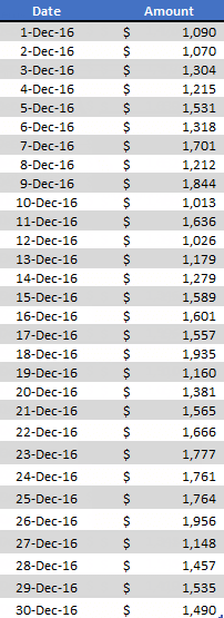
Below, I have a table with day-wise sales, and I want to highlight the top 10 days with the highest sales (the table is a bit long here).
Highlight Top 10 Values
- First of all, select the data from which you want to highlight top values.
- Go to Home Tab -> Styles -> Conditional Formatting -> Top/Bottom Rules -> Top 10 Items.
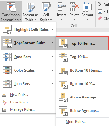
- Now, in the pop-up window, you have two things to specify.
- The number of values to highlight (top 10 for now).
- Formatting to use for highlighting values.
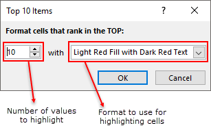
- After that, click OK.

It will instantly highlight the top 10 values from the data with the formatting style you have selected. If there’s a tie at the 10th place, all the tied values are highlighted, so you may see more than 10 cells.
Highlight Bottom 10 Values
For highlighting the bottom 10 values, you can use the same steps. But instead of Top 10 Items, just click on Bottom 10 Items, and the rest of the steps are the same.
- Select the number of values to highlight.
- And the format to use.
What Else?
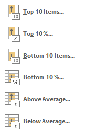
In the Top/Bottom Rules option in conditional formatting, you have some other useful options.
- Top 10% – Use this to highlight the top 10% of the cells (for 200 values, the 20 highest).
- Bottom 10% – Highlight the bottom 10% of the cells.
- Above Average – For highlighting values that are above the average value of the data.
- Below Average – Use this to highlight values that are below the average value of the data.
As I already said, I highlight top and bottom values in all my reports. And this also helps the other person get a quick insight, even if the data is just a table.
Highlight the Entire Row of the Top Values
The built-in rule only colors the cells with the values. To highlight the whole row (like the date and the sales), use a formula rule with LARGE. Select the full table (like A2:B100), go to Home ➜ Conditional Formatting ➜ New Rule ➜ Use a formula to determine which cells to format, and enter:
=$B2>=LARGE($B$2:$B$100,10)
To make the number of top values flexible, type it in a cell (like E1) and use that cell instead of 10. Change E1, and the highlight changes with it:
=$B2>=LARGE($B$2:$B$100,$E$1)
And for the bottom values, use SMALL. The first part skips blank cells, which SMALL would otherwise treat as the lowest:
=AND($B2<>"",$B2<=SMALL($B$2:$B$100,$E$1))
List the Top Values with a Formula
If you also want the top values in a separate list, use LARGE with 1 for the highest value, 2 for the second highest, and so on:
=LARGE($B$2:$B$100,1)
In Excel 2021 and Microsoft 365, you can get the whole top 10 in one go with SEQUENCE, and the results spill down:
=LARGE($B$2:$B$100,SEQUENCE(10))
Frequently Asked Questions
Why are more than 10 cells highlighted?
Because some values are tied. If the 10th and 11th highest values are the same, Excel highlights both.
Can I highlight top and bottom values in the same range?
Yes. Apply a Top 10 Items rule and then a Bottom 10 Items rule to the same range, each with its own color (like green and red).
Does the highlight update when the data changes?
Yes. Conditional formatting recalculates with the data, so the highlight moves to the new top or bottom values as soon as you change them.
Hi… sir please answer me one thing that on what principal or formula top 10% or bottom 10% work and if we take 20% instead of 10% then what happens.