Excel VBA Macro Codes: Ready-to-Use Examples
Last Updated: 27th April 2026 by Puneet Gogia
Jump to a Category
 Cells & Ranges10 codes
 Formatting & Highlighting20 codes
 Text & String Operations10 codes
 Numbers & Dates19 codes
 Worksheet Management16 codes
 Workbook & File Management11 codes
 Printing & PDF Export5 codes
 Charts & Pivot Tables9 codes
 Automation & Utilities16 codes
Macro codes can save you a ton of time. You can automate small as well as heavy tasks with VBA codes. And do you know? With the help of macros, you can break all the limitations of Excel which you think Excel has. And today, I have listed some of the useful codes examples to help you become more productive in your day to day work. You can use these codes even if you haven’t used VBA before that.
But here’s the first thing to know:
What is a Macro (VBA Code) ?
In Excel, macro code is a programming code which is written in VBA (Visual Basic for Applications) language. The idea behind using a macro code is to automate an action which you perform manually in Excel, otherwise. For example, you can use a code to print only a particular range of cells just with a single click instead of selecting the range > File Tab > Print > Print Select > OK Button.
How to use a Macro in Excel (VBA Code)?
Before you use these codes, make sure you have your developer tab on your Excel ribbon to access VB editor. Once you activate developer tab you can use below steps to paste a VBA code into VB editor.
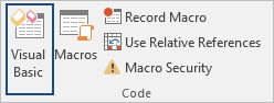
- Go to your developer tab and click on "Visual Basic" to open the Visual Basic Editor.
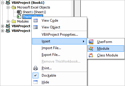
- On the left side in "Project Window", right click on the name of your workbook and insert a new module.
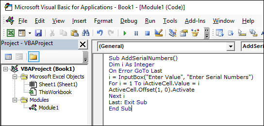
- Just paste your code into the module and close it.
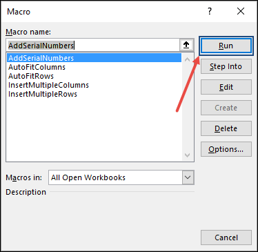
- Now, go to your developer tab and click on the macro button.
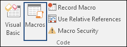
- It will show you a window with a list of the macros you have in your file from where you can run a macro from that list.
All codes on this page have been tested in Excel 2016, 2019, 2021, 2024, and Microsoft 365 on Windows. Before using any macro, keep in mind:
- Save your workbook as .xlsm (macro-enabled) before running any code, .xlsx files cannot store macros.
- Codes marked Windows only use Shell commands or Outlook automation that do not work on Mac.
- To use macros in all your workbooks, save them to your Personal Macro Workbook.
- Always test a macro on a copy of your file first — some operations like deleting sheets or replacing values cannot be undone.
Add Serial Numbers
Automatically adds a sequential list of numbers downward from the active cell. An input box asks how many numbers to insert.
Sub AddSerialNumbers()
    Dim i As Integer
    On Error GoTo Last
    i = InputBox("Enter Value", "Enter Serial Numbers")
    For i = 1 To i
        ActiveCell.Value = i
        ActiveCell.Offset(1, 0).Activate
    Next i
Last: Exit Sub
End SubInsert Multiple Columns
Inserts a specified number of columns to the right of the active cell in one step — no need to repeat the insert command manually.
Sub InsertMultipleColumns()
    Dim i As Integer, j As Integer
    ActiveCell.EntireColumn.Select
    On Error GoTo Last
    i = InputBox("Enter number of columns to insert", "Insert Columns")
    For j = 1 To i
        Selection.Insert Shift:=xlToRight, CopyOrigin:=xlFormatFromRightorAbove
    Next j
Last: Exit Sub
End SubxlToRight to xlToLeft to insert columns before the selected cell instead.Insert Multiple Rows
Inserts multiple rows at once starting from the active cell. Enter the count in the input box when prompted.
Sub InsertMultipleRows()
    Dim i As Integer, j As Integer
    ActiveCell.EntireRow.Select
    On Error GoTo Last
    i = InputBox("Enter number of rows to insert", "Insert Rows")
    For j = 1 To i
        Selection.Insert Shift:=xlToDown, CopyOrigin:=xlFormatFromRightorAbove
    Next j
Last: Exit Sub
End SubxlToDown to xlToUp to insert rows above the selected cell.Auto Fit Columns
Instantly auto-fits the width of every column in the active worksheet to match its content — no manual dragging needed.
Sub AutoFitColumns()
    Cells.Select
    Cells.EntireColumn.AutoFit
End Sub
Auto Fit Rows
Instantly auto-fits the height of every row in the active worksheet to match its content.
Sub AutoFitRows()
    Cells.Select
    Cells.EntireRow.AutoFit
End Sub
Remove Text Wrap (Entire Sheet)
Range("A1").WrapText = False which only removed wrap from cell A1. Now correctly applies to the entire sheet.Removes text wrap from every cell in the active worksheet, then auto-fits all rows and columns so your layout snaps back into shape.
Sub RemoveTextWrap()
    Cells.WrapText = False
    Cells.EntireRow.AutoFit
    Cells.EntireColumn.AutoFit
End SubCells with e.g. Range("A1:D50").Unmerge Cells
Unmerges all merged cells in the current selection. Add to your Quick Access Toolbar for one-click access.
Sub UnmergeCells()
    Selection.UnMerge
End SubSelection with a fixed range like Range("A1:D10") to target a specific area.Unhide All Rows and Columns
Makes all hidden rows and columns in the active worksheet visible again — no need to unhide them one by one.
Sub UnhideRowsColumns()
    Columns.EntireColumn.Hidden = False
    Rows.EntireRow.Hidden = False
End Sub
Convert Range into a Static Image
Copies the selected range and pastes it as a static picture into the same sheet. Useful for locking down a table's appearance for reporting.
Sub PasteAsPicture()
    Application.CutCopyMode = False
    Selection.Copy
    ActiveSheet.Pictures.Paste.Select
End Sub
Insert a Linked Picture
Pastes the selected range as a linked image — the picture updates automatically when the source data changes. Great for dashboards.
Sub LinkedPicture()
    Selection.Copy
    ActiveSheet.Pictures.Paste(Link:=True).Select
End SubTo manage all of these codes, make sure to read about the Personal Macro Workbook so that you can use them in all the workbooks.
Highlight Duplicate Values
Checks each cell in the selection and highlights any duplicate values in yellow. Select your range before running.
Sub HighlightDuplicateValues()
    Dim myRange As Range, myCell As Range
    Set myRange = Selection
    For Each myCell In myRange
        If WorksheetFunction.CountIf(myRange, myCell.Value) > 1 Then
            myCell.Interior.ColorIndex = 36
        End If
    Next myCell
End SubColorIndex = 36 to any Excel color index number to use a different highlight colour.Highlight Active Row and Column on Double-Click
Double-click any cell to select its entire row and column — great for navigating large data tables. This goes in the sheet's own code window, not a module.
Private Sub Worksheet_BeforeDoubleClick(ByVal Target As Range, Cancel As Boolean)
    Dim strRange As String
    strRange = Target.Cells.Address & "," & _
               Target.Cells.EntireColumn.Address & "," & _
               Target.Cells.EntireRow.Address
    Range(strRange).Select
End SubHighlight Top 10 Values
Select a range and run this macro to highlight the top 10 values in green using a conditional formatting rule.
Sub HighlightTopTen()
    Selection.FormatConditions.AddTop10
    Selection.FormatConditions(Selection.FormatConditions.Count).SetFirstPriority
    With Selection.FormatConditions(1)
        .TopBottom = xlTop10Top
        .Rank = 10
        .Percent = False
    End With
    With Selection.FormatConditions(1).Interior
        .Color = 13561798
    End With
    Selection.FormatConditions(1).StopIfTrue = False
End Sub.Rank = 10 to highlight more or fewer values. Change xlTop10Top to xlTop10Bottom for the lowest values.Highlight Named Ranges
Highlights all named ranges in the workbook so you can see exactly which cells have names assigned to them.
Sub HighlightNamedRanges()
    Dim RangeName As Name, HighlightRange As Range
    On Error Resume Next
    For Each RangeName In ActiveWorkbook.Names
        Set HighlightRange = RangeName.RefersToRange
        HighlightRange.Interior.ColorIndex = 36
    Next RangeName
End Sub
Highlight Cells Greater Than a Value
Prompts for a threshold and highlights all cells in the selection that are greater than it in green.
Sub HighlightGreaterThanValues()
    Dim i As Integer
    i = InputBox("Enter Greater Than Value", "Enter Value")
    Selection.FormatConditions.Delete
    Selection.FormatConditions.Add Type:=xlCellValue, Operator:=xlGreater, Formula1:=i
    Selection.FormatConditions(Selection.FormatConditions.Count).SetFirstPriority
    With Selection.FormatConditions(1)
        .Font.Color = RGB(0, 0, 0)
        .Interior.Color = RGB(31, 218, 154)
    End With
End Sub
Highlight Cells Lower Than a Value
Prompts for a threshold and highlights all cells in the selection that are below it in red.
Sub HighlightLowerThanValues()
    Dim i As Integer
    i = InputBox("Enter Lower Than Value", "Enter Value")
    Selection.FormatConditions.Delete
    Selection.FormatConditions.Add Type:=xlCellValue, Operator:=xlLess, Formula1:=i
    Selection.FormatConditions(Selection.FormatConditions.Count).SetFirstPriority
    With Selection.FormatConditions(1)
        .Font.Color = RGB(0, 0, 0)
        .Interior.Color = RGB(217, 83, 79)
    End With
End Sub
Highlight Negative Numbers
Scans every cell in the selection and changes the font colour of any negative number to red.
Sub HighlightNegativeNumbers()
    Dim Rng As Range
    For Each Rng In Selection
        If WorksheetFunction.IsNumber(Rng) Then
            If Rng.Value < 0 Then
                Rng.Font.Color = -16776961
            End If
        End If
    Next
End Sub
Highlight Specific Text within Cells
Searches for a specific text string and highlights matching characters in red. Select two columns before running: column A = source text, column B = the text to find.
Sub HighlightSpecificText()
    Dim myStr As String, myRg As Range
    Dim I As Long, J As Long
    On Error Resume Next
    Set myRg = Application.InputBox("Select a two-column range:", "Selection Required", , , , , , 8)
    If myRg Is Nothing Then Exit Sub
    If myRg.Columns.Count <> 2 Then
        MsgBox "Please select exactly two columns." : Exit Sub
    End If
    For I = 0 To myRg.Rows.Count - 1
        myStr = myRg.Range("B1").Offset(I, 0).Value
        With myRg.Range("A1").Offset(I, 0)
            .Font.ColorIndex = 1
            For J = 1 To Len(.Text)
                If Mid(.Text, J, Len(myStr)) = myStr Then
                    .Characters(J, Len(myStr)).Font.ColorIndex = 3
                End If
            Next J
        End With
    Next I
End Sub
Highlight Cells with Comments
Applies the built-in "Note" style to all cells containing comments in the current selection, making them easy to spot at a glance.
Sub HighlightCommentCells()
    Selection.SpecialCells(xlCellTypeComments).Select
    Selection.Style = "Note"
End Sub
Highlight Alternate Rows (Banded/Striped)
rng.Value = rng ^ (1/3) which permanently replaced cell values with their cube roots. That line has been removed.Highlights every other row in the selection to create a striped/banded table effect that makes data easier to read.
Sub HighlightAlternateRows()
    Dim rng As Range
    For Each rng In Selection.Rows
        If rng.Row Mod 2 = 1 Then
            rng.Style = "20% - Accent1"
        End If
    Next rng
End Sub"20% - Accent1" to Accent2–Accent6 for different colours. Change Mod 2 = 1 to Mod 2 = 0 to highlight even rows instead.Highlight Cells with Misspelled Words
Scans the entire used range and applies the "Bad" style to any cell containing a spelling error.
Sub HighlightMisspelledCells()
    Dim rng As Range
    For Each rng In ActiveSheet.UsedRange
        If Not Application.CheckSpelling(Word:=rng.Text) Then
            rng.Style = "Bad"
        End If
    Next rng
End Sub
Highlight All Error Cells
Scans the entire worksheet, highlights all error cells in red, and shows a count of how many were found.
Sub HighlightErrors()
    Dim rng As Range, i As Integer
    For Each rng In ActiveSheet.UsedRange
        If WorksheetFunction.IsError(rng) Then
            i = i + 1
            rng.Style = "Bad"
        End If
    Next rng
    MsgBox "There are total " & i & " error(s) in this worksheet."
End Sub
Highlight Cells with Specific Text
Prompts for a value, then highlights every matching cell in the used range and shows a count of matches found.
Sub HighlightSpecificValues()
    Dim rng As Range, i As Integer, c As Variant
    c = InputBox("Enter Value To Highlight")
    For Each rng In ActiveSheet.UsedRange
        If rng = c Then
            rng.Style = "Note"
            i = i + 1
        End If
    Next rng
    MsgBox "There are total " & i & " " & c & " in this worksheet."
End Sub
Highlight Blank Cells with Hidden Spaces
Finds cells that look blank but contain a single space character — a common data quality issue — and highlights them.
Sub HighlightBlankWithSpace()
    Dim rng As Range
    For Each rng In ActiveSheet.UsedRange
        If rng.Value = " " Then
            rng.Style = "Note"
        End If
    Next rng
End Sub
Highlight Maximum Value in Selection
Finds the highest value in the selected range and highlights it in green.
Sub HighlightMaxValue()
    Dim rng As Range
    For Each rng In Selection
        If rng = WorksheetFunction.Max(Selection) Then
            rng.Style = "Good"
        End If
    Next rng
End Sub
Highlight Minimum Value in Selection
Finds the lowest value in the selected range and highlights it in green.
Sub HighlightMinValue()
    Dim rng As Range
    For Each rng In Selection
        If rng = WorksheetFunction.Min(Selection) Then
            rng.Style = "Good"
        End If
    Next rng
End Sub
Highlight Unique Values
Highlights all cells in the selection that contain a unique (non-duplicate) value using a conditional formatting rule.
Sub HighlightUniqueValues()
    Dim rng As Range
    Set rng = Selection
    rng.FormatConditions.Delete
    Dim uv As UniqueValues
    Set uv = rng.FormatConditions.AddUniqueValues
    uv.DupeUnique = xlUnique
    uv.Interior.Color = vbGreen
End Sub
Highlight Column Differences
Highlights cells where the value differs from the corresponding cell in the reference column — ideal for comparing two data sets side by side.
Sub ColumnDifference()
    Selection.ColumnDifferences(ActiveCell).Select
    Selection.Style = "Bad"
End SubHighlight Row Differences
Highlights cells where the value differs from the corresponding cell in the reference row.
Sub RowDifference()
    Selection.RowDifferences(ActiveCell).Select
    Selection.Style = "Bad"
End Sub
Lock / Protect Cells with Formulas
Protects only formula cells, leaving all other cells editable. Useful for sharing workbooks where you want to prevent accidental formula deletion.
Sub LockCellsWithFormulas()
    With ActiveSheet
        .Unprotect
        .Cells.Locked = False
        .Cells.SpecialCells(xlCellTypeFormulas).Locked = True
        .Protect AllowDeletingRows:=True
    End With
End Sub
Highlight All Formula Cells
Scans the entire used range and highlights every cell containing a formula in yellow — useful for quickly auditing a sheet.
Sub HighlightFormulas()
    Dim cell As Range
    For Each cell In ActiveSheet.UsedRange
        If cell.HasFormula Then
            cell.Interior.Color = RGB(255, 255, 0)
        End If
    Next cell
End SubConvert to UPPER CASE
Converts all text in the selected cells to UPPER CASE. Non-text cells are left unchanged.
Sub ConvertToUpperCase()
    Dim Rng As Range
    For Each Rng In Selection
        If Application.WorksheetFunction.IsText(Rng) Then
            Rng.Value = UCase(Rng)
        End If
    Next
End Sub
Convert to lower case
Converts all text in the selected cells to lower case. Non-text cells are skipped.
Sub ConvertToLowerCase()
    Dim Rng As Range
    For Each Rng In Selection
        If Application.WorksheetFunction.IsText(Rng) Then
            Rng.Value = LCase(Rng)
        End If
    Next
End Sub
Convert to Proper Case
Capitalises The First Letter Of Every Word. Useful for cleaning name lists or titles.
Sub ConvertToProperCase()
    Dim Rng As Range
    For Each Rng In Selection
        If WorksheetFunction.IsText(Rng) Then
            Rng.Value = WorksheetFunction.Proper(Rng.Value)
        End If
    Next
End Sub
Convert to Sentence case
Capitalises only the first letter of the text in each cell. Perfect for sentence-style labels and descriptions.
Sub ConvertToSentenceCase()
    Dim Rng As Range
    For Each Rng In Selection
        If WorksheetFunction.IsText(Rng) Then
            Rng.Value = UCase(Left(Rng, 1)) & LCase(Right(Rng, Len(Rng) - 1))
        End If
    Next Rng
End Sub
Remove Extra Spaces from Cells
Trims leading, trailing, and extra internal spaces from every text cell in the selection — equivalent to applying Excel's TRIM function directly to the values.
Sub RemoveSpaces()
    Dim myCell As Range
    Select Case MsgBox("You Can't Undo This. Save Workbook First?", vbYesNoCancel, "Alert")
        Case Is = vbYes:    ThisWorkbook.Save
        Case Is = vbCancel: Exit Sub
    End Select
    For Each myCell In Selection
        If Not IsEmpty(myCell) Then myCell = Trim(myCell)
    Next myCell
End Sub
Remove First N Characters (Custom Function)
A custom worksheet function that removes a specified number of characters from the start of a text string. Use it in a cell like a regular formula.
Public Function RemoveFirstC(rng As String, cnt As Long)
    RemoveFirstC = Right(rng, Len(rng) - cnt)
End Function=RemoveFirstC(A1, 3) removes the first 3 characters from A1. Paste into a module to use as a worksheet function.Remove a Specific Character from Selection
Prompts you to enter a character and removes every instance of it from all cells in the selection.
Sub RemoveChar()
    Dim Rng As Range, rc As String
    rc = InputBox("Character(s) to Remove", "Enter Value")
    For Each Rng In Selection
        Selection.Replace What:=rc, Replacement:=""
    Next
End Sub
Reverse Text in a Cell (Custom Function)
A custom worksheet function that reverses the characters in a text string. Use it directly in cells like any Excel formula.
Public Function Rvrse(ByVal cell As Range) As String
    Rvrse = VBA.StrReverse(cell.Value)
End Function=Rvrse(A1) where A1 contains "Excel" returns "lecxE".Count Total Words in a Worksheet
Counts every word across all cells in the active worksheet and displays the total in a message box.
Sub WordCountWorksheet()
    Dim WordCnt As Long, rng As Range
    Dim S As String, N As Long
    For Each rng In ActiveSheet.UsedRange.Cells
        S = Application.WorksheetFunction.Trim(rng.Text)
        N = 0
        If S <> vbNullString Then
            N = Len(S) - Len(Replace(S, " ", "")) + 1
        End If
        WordCnt = WordCnt + N
    Next rng
    MsgBox "There are total " & Format(WordCnt, "#,##0") & " words in the active worksheet"
End Sub
Convert Numbers to Words (Custom Function)
A custom worksheet function that converts any whole number to its written English equivalent. Use it in cells like a regular Excel formula: =NumberToWords(A1).
Function NumberToWords(ByVal MyNumber As Long) As String
    Dim Units(1 To 9) As String, Teens(10 To 19) As String
    Dim Tens(2 To 9) As String, Result As String
    Units(1)="One":Units(2)="Two":Units(3)="Three":Units(4)="Four"
    Units(5)="Five":Units(6)="Six":Units(7)="Seven"
    Units(8)="Eight":Units(9)="Nine"
    Teens(10)="Ten":Teens(11)="Eleven":Teens(12)="Twelve"
    Teens(13)="Thirteen":Teens(14)="Fourteen":Teens(15)="Fifteen"
    Teens(16)="Sixteen":Teens(17)="Seventeen"
    Teens(18)="Eighteen":Teens(19)="Nineteen"
    Tens(2)="Twenty":Tens(3)="Thirty":Tens(4)="Forty"
    Tens(5)="Fifty":Tens(6)="Sixty":Tens(7)="Seventy"
    Tens(8)="Eighty":Tens(9)="Ninety"
    If MyNumber = 0 Then NumberToWords = "Zero": Exit Function
    If MyNumber < 0 Then Result = "Negative ": MyNumber = Abs(MyNumber)
    If MyNumber >= 1000 Then
        Result = Result & Units(Int(MyNumber/1000)) & " Thousand "
        MyNumber = MyNumber Mod 1000
    End If
    If MyNumber >= 100 Then
        Result = Result & Units(Int(MyNumber/100)) & " Hundred "
        MyNumber = MyNumber Mod 100
    End If
    If MyNumber >= 20 Then
        Result = Result & Tens(Int(MyNumber/10)) & " "
        MyNumber = MyNumber Mod 10
    ElseIf MyNumber >= 10 Then
        Result = Result & Teens(MyNumber): MyNumber = 0
    End If
    If MyNumber > 0 Then Result = Result & Units(MyNumber)
    NumberToWords = Trim(Result)
End Function=NumberToWords(1234) returns "One Thousand Two Hundred Thirty Four". Works for −9,999 to 9,999.Multiply All Values by a Number
Multiplies every number in the selection by a value you specify. The original code used addition (+) instead of multiplication (*) — now fixed. Also upgraded to Double so decimal multipliers like 1.5 work correctly.
Sub MultiplyAllValues()
    Dim rng As Range, i As Double
    i = InputBox("Enter the number to multiply by", "Multiply Values")
    If i = 0 Then Exit Sub
    For Each rng In Selection
        If WorksheetFunction.IsNumber(rng) Then
            rng.Value = rng.Value * i
        End If
    Next rng
End Sub2 to double all values, 0.5 to halve them, or 1.1 to add 10%. Non-numeric cells are skipped automatically.Add a Number to All Values
Adds the same number to every cell in the selection. Enter a negative value (e.g. -10) to subtract from all values instead. Useful for bulk adjustments like adding a fixed fee or offset across a list of prices.
Sub AddToAllValues()
    Dim rng As Range, i As Double
    i = InputBox("Enter the number to add", "Add to Values")
    For Each rng In Selection
        If WorksheetFunction.IsNumber(rng) Then
            rng.Value = rng.Value + i
        End If
    Next rng
End Sub-10 to subtract 10 from every cell. Non-numeric cells are ignored.Calculate Square Root of All Values
Replaces every number in the selection with its square root, in-place — no helper column needed. Useful for bulk statistical transformations on a dataset.
Sub GetSquareRoot()
    Dim rng As Range
    For Each rng In Selection
        If WorksheetFunction.IsNumber(rng) Then
            rng.Value = Sqr(rng)
        End If
    Next rng
End Sub
Calculate Cube Root of All Values
Replaces every number in the selection with its cube root. Uses the exponent ^ (1/3) since VBA has no built-in cube root function.
Sub GetCubeRoot()
    Dim rng As Range
    For Each rng In Selection
        If WorksheetFunction.IsNumber(rng) Then
            rng.Value = rng ^ (1 / 3)
        End If
    Next rng
End Sub
Remove Decimals from Numbers
Strips the decimal portion from every number in the selection, rounding down to the nearest whole number using VBA's Int() function.
Sub RemoveDecimals()
    Dim rng As Range
    For Each rng In Selection
        rng.Value = Int(rng)
        rng.NumberFormat = "0"
    Next rng
End SubInt() always rounds down (toward negative infinity). 2.9 becomes 2, -2.1 becomes -3. Use Round(rng, 0) instead if you want standard rounding.Remove Negative Signs (Convert to Absolute Values)
Converts all negative numbers in the selection to their absolute (positive) values using VBA's Abs() function. Non-numeric cells are skipped.
Sub RemoveNegativeSign()
    Dim rng As Range
    For Each rng In Selection
        If WorksheetFunction.IsNumber(rng) Then
            rng.Value = Abs(rng)
        End If
    Next rng
End Sub
Remove Apostrophe from Numbers
Removes leading apostrophes from numbers stored as text — a common problem when importing data from other systems. The apostrophe forces Excel to treat the number as text; this macro converts them back to true numeric values.
Sub RemoveApostrophes()
    Selection.Value = Selection.Value
End SubReplace Blank Cells with Zero
Finds every empty cell (including cells with a single space) in the selection and fills it with 0. Prevents #DIV/0! and other formula errors that occur when calculations reference blank cells.
Sub ReplaceBlankWithZero()
    Dim rng As Range
    For Each rng In Selection
        If rng = "" Or rng = " " Then
            rng.Value = "0"
        End If
    Next rng
End Sub
Convert Roman Numerals to Arabic Numbers
Converts Roman numeral text (e.g. XIV, XLII) in selected cells to their Arabic number equivalents using Excel's built-in ARABIC worksheet function.
Sub ConvertRomanToArabic()
    Dim rng As Range
    For Each rng In Selection
        If Not WorksheetFunction.IsNonText(rng) Then
            rng.Value = WorksheetFunction.Arabic(rng)
        End If
    Next rng
End SubAdd Degree Symbol to Numbers
Appends a degree symbol (°) to every number in the selection. Useful for temperature data, angles, or any measurement that requires the degree symbol but where you want to keep the values editable.
Sub AddDegreeSymbol()
    Dim rng As Range
    For Each rng In Selection
        If IsNumeric(rng.Value) Then
            rng.Value = rng.Value & "°"
        End If
    Next
End Sub"0°") instead.Convert All Formulas to Static Values
Replaces every formula in the selection with its current calculated value — permanently locking in results and removing formula dependencies. A save prompt appears first because this action cannot be undone.
Sub ConvertToValues()
    Dim MyRange As Range, MyCell As Range
    Select Case MsgBox("You Can't Undo This. Save Workbook First?", vbYesNoCancel, "Alert")
        Case Is = vbYes:    ThisWorkbook.Save
        Case Is = vbCancel: Exit Sub
    End Select
    Set MyRange = Selection
    For Each MyCell In MyRange
        If MyCell.HasFormula Then
            MyCell.Formula = MyCell.Value
        End If
    Next MyCell
End Sub
Convert Dates to Day Numbers
Extracts the day number from each date in the selection and replaces the date with just the day (e.g. 25-Dec-2024 becomes 25). Useful for grouping or filtering data by day of month.
Sub DateToDay()
    Dim tempCell As Range
    For Each tempCell In Selection
        If IsDate(tempCell) = True Then
            With tempCell
                .Value = Day(tempCell)
                .NumberFormat = "0"
            End With
        End If
    Next tempCell
End Sub
Convert Dates to Year Numbers
Extracts just the year from each date in the selection (e.g. 25-Dec-2024 becomes 2024). Useful for year-based grouping in reports or pivot tables.
Sub DateToYear()
    Dim tempCell As Range
    For Each tempCell In Selection
        If IsDate(tempCell) = True Then
            With tempCell
                .Value = Year(tempCell)
                .NumberFormat = "0"
            End With
        End If
    Next tempCell
End Sub
Remove Time from Date-Time Values
Strips the time portion from cells that contain a combined date and time value, leaving just the date. Uses VBA.Int() to drop the decimal (time) part of the serial number.
Sub RemoveTime()
    Dim Rng As Range
    For Each Rng In Selection
        If IsDate(Rng) = True Then
            Rng.Value = VBA.Int(Rng.Value)
        End If
    Next
    Selection.NumberFormat = "dd-mmm-yy"
End Sub"dd-mmm-yy" to your preferred date format, e.g. "dd/mm/yyyy" or "mm/dd/yyyy".Remove Date from Date-Time Values
Strips the date from combined date-time cells, returning only the time value. Uses VBA.Fix() to subtract the integer (date) part and keep just the decimal (time) portion.
Sub RemoveDate()
    Dim Rng As Range
    For Each Rng In Selection
        If IsDate(Rng) = True Then
            Rng.Value = Rng.Value - VBA.Fix(Rng.Value)
        End If
    Next
    Selection.NumberFormat = "hh:mm:ss am/pm"
End Sub
Insert a 24-Hour Time Range
Inserts a full 24-hour time sequence (1:00 AM through 12:00 AM) starting from the active cell, one hour per row going downward. Useful for building time-based schedules or logs.
Sub InsertTimeRange()
    Dim i As Integer
    For i = 1 To 24
        ActiveCell.FormulaR1C1 = i & ":00"
        ActiveCell.NumberFormat = "[$-409]h:mm AM/PM;@"
        ActiveCell.Offset(RowOffset:=1, ColumnOffset:=0).Select
    Next i
End SubInsert A–Z Alphabets in a Range
Inserts the full alphabet (A–Z or a–z) starting from the active cell, one letter per row. Two versions provided — uppercase and lowercase. Uses ASCII character codes with Chr().
' Uppercase A-Z
Sub InsertUppercaseAlphabets()
    Dim i As Integer
    For i = 65 To 90
        ActiveCell.Value = Chr(i)
        ActiveCell.Offset(1, 0).Select
    Next i
End Sub

' Lowercase a-z
Sub InsertLowercaseAlphabets()
    Dim i As Integer
    For i = 97 To 122
        ActiveCell.Value = Chr(i)
        ActiveCell.Offset(1, 0).Select
    Next i
End Sub
Switch Between A1 and R1C1 Reference Styles
Toggles between Excel's A1 (column letters + row numbers) and R1C1 (row and column numbers) reference styles without going into Excel Options. Run the matching Sub for the style you want.
' Switch to R1C1 style
Sub ActivateR1C1()
    Application.ReferenceStyle = xlR1C1
End Sub

' Switch back to A1 style
Sub ActivateA1()
    Application.ReferenceStyle = xlA1
End SubActivate R1C1 / A1 Reference Style (Shortcut)
A combined toggle macro — checks the current reference style and switches to the other one automatically. Run once to switch to R1C1, run again to switch back to A1.
Sub ToggleReferenceStyle()
    If Application.ReferenceStyle = xlA1 Then
        Application.ReferenceStyle = xlR1C1
        MsgBox "Switched to R1C1 reference style.", vbInformation
    Else
        Application.ReferenceStyle = xlA1
        MsgBox "Switched to A1 reference style.", vbInformation
    End If
End SubInsert Multiple Worksheets at Once
Adds multiple new worksheets after the active sheet in one step. Enter the count when prompted.
Sub InsertMultipleSheets()
    Dim i As Integer
    i = InputBox("Enter number of sheets to insert.", "Insert Multiple Sheets")
    Sheets.Add After:=ActiveSheet, Count:=i
End Sub
Hide All Sheets Except the Active One
Hides every worksheet in the workbook except the one you're currently viewing.
Sub HideAllButActiveSheet()
    Dim ws As Worksheet
    For Each ws In ThisWorkbook.Worksheets
        If ws.Name <> ThisWorkbook.ActiveSheet.Name Then
            ws.Visible = xlSheetHidden
        End If
    Next ws
End Sub
Unhide All Hidden Worksheets
Makes all hidden sheets in the workbook visible again with a single click.
Sub UnhideAllWorksheets()
    Dim ws As Worksheet
    For Each ws In ActiveWorkbook.Worksheets
        ws.Visible = xlSheetVisible
    Next ws
End Sub
Delete All Sheets Except the Active One
Permanently deletes every worksheet except the currently active one. Cannot be undone — save first.
Sub DeleteAllButActiveSheet()
    Dim ws As Worksheet
    For Each ws In ThisWorkbook.Worksheets
        If ws.Name <> ThisWorkbook.ActiveSheet.Name Then
            Application.DisplayAlerts = False
            ws.Delete
            Application.DisplayAlerts = True
        End If
    Next ws
End Sub
Delete All Blank Worksheets
Scans every sheet in the workbook and deletes any that are completely empty.
Sub DeleteBlankWorksheets()
    Dim Ws As Worksheet
    On Error Resume Next
    Application.ScreenUpdating = False
    Application.DisplayAlerts = False
    For Each Ws In Application.Worksheets
        If Application.WorksheetFunction.CountA(Ws.UsedRange) = 0 Then
            Ws.Delete
        End If
    Next
    Application.ScreenUpdating = True
    Application.DisplayAlerts = True
End Sub
Protect a Worksheet
Protects the active worksheet with a password. Edit the password directly in the code before running.
Sub ProtectWorksheet()
    ActiveSheet.Protect "mypassword", True, True
End Sub"mypassword" with your actual password before running.Unprotect a Worksheet
Removes protection from the active worksheet using the password set in the code.
Sub UnprotectWorksheet()
    ActiveSheet.Unprotect "mypassword"
End Sub
Protect All Worksheets at Once
Prompts for a password and applies it to every worksheet in the workbook simultaneously.
Sub ProtectAllWorksheets()
    Dim ws As Worksheet, ps As String
    ps = InputBox("Enter a Password.", vbOKCancel)
    For Each ws In ActiveWorkbook.Worksheets
        ws.Protect Password:=ps
    Next ws
End Sub
Protect All Sheets with Confirmation
Password-protects every sheet in the workbook at once. An input box lets you set the password on the fly — no need to hardcode it.
Sub ProtectAllSheets()
    Dim ws As Worksheet, pwd As String
    pwd = InputBox("Enter a password to protect all sheets", "Protect Sheets")
    If pwd = "" Then Exit Sub
    For Each ws In ThisWorkbook.Sheets
        ws.Protect Password:=pwd
    Next ws
    MsgBox "All sheets are now protected.", vbInformation
End SubUnprotect All Sheets in a Workbook
Removes password protection from every sheet in the workbook at once.
Sub UnprotectAllSheets()
    Dim ws As Worksheet
    For Each ws In ThisWorkbook.Sheets
        ws.Unprotect Password:="password"
    Next ws
End Sub"password" with the password used when protecting the sheets.Sort Worksheets Alphabetically
Sorts all worksheets alphabetically. A message box lets you choose ascending or descending order.
Sub SortWorksheets()
    Dim i As Integer, j As Integer, iAnswer As VbMsgBoxResult
    iAnswer = MsgBox("Sort Ascending? Click No for Descending.", vbYesNoCancel + vbQuestion, "Sort Worksheets")
    For i = 1 To Sheets.Count
        For j = 1 To Sheets.Count - 1
            If iAnswer = vbYes Then
                If UCase$(Sheets(j).Name) > UCase$(Sheets(j+1).Name) Then
                    Sheets(j).Move After:=Sheets(j+1)
                End If
            ElseIf iAnswer = vbNo Then
                If UCase$(Sheets(j).Name) < UCase$(Sheets(j+1).Name) Then
                    Sheets(j).Move After:=Sheets(j+1)
                End If
            End If
        Next j
    Next i
End Sub
Create a Table of Contents for All Sheets
Creates a new "Table of Content" sheet with a clickable hyperlink to every other sheet in the workbook — essential for large multi-sheet files.
Sub TableOfContent()
    Dim i As Long
    On Error Resume Next
    Application.DisplayAlerts = False
    Worksheets("Table of Content").Delete
    Application.DisplayAlerts = True
    On Error GoTo 0
    ThisWorkbook.Sheets.Add Before:=ThisWorkbook.Worksheets(1)
    ActiveSheet.Name = "Table of Content"
    For i = 1 To Sheets.Count
        With ActiveSheet
            .Hyperlinks.Add Anchor:=ActiveSheet.Cells(i, 1), _
                Address:="", _
                SubAddress:="'" & Sheets(i).Name & "'!A1", _
                ScreenTip:=Sheets(i).Name, _
                TextToDisplay:=Sheets(i).Name
        End With
    Next i
End Sub
Save Each Worksheet as a Separate PDF
Exports every worksheet in the workbook as its own PDF file. Update the folder path in the code before running.
Sub SaveEachSheetAsPDF()
    Dim ws As Worksheet
    For Each ws In Worksheets
        ws.ExportAsFixedFormat xlTypePDF, "C:\YourFolder\" & ws.Name & ".pdf"
    Next ws
End Sub"C:\YourFolder\" with your actual save location.Insert Blank Rows Between Each Existing Row
Inserts 2 blank rows after every existing row — useful for adding spacing in reports or room for annotations.
Sub InsertRowsBetweenRows()
    Dim i As Long
    For i = ThisWorkbook.Sheets("Sheet1").UsedRange.Rows.Count To 1 Step -1
        ThisWorkbook.Sheets("Sheet1").Rows(i + 1).Resize(2).Insert
    Next i
End Sub"Sheet1" to your sheet name. Change Resize(2) to insert a different number of blank rows.Disable Page Breaks Across All Workbooks
Turns off the page break display on all worksheets across all open workbooks — cleans up the view after printing.
Sub DisablePageBreaks()
    Dim wb As Workbook, Sht As Worksheet
    Application.ScreenUpdating = False
    For Each wb In Application.Workbooks
        For Each Sht In wb.Worksheets
            Sht.DisplayPageBreaks = False
        Next Sht
    Next wb
    Application.ScreenUpdating = True
End Sub
Auto Sort Data in a Worksheet
Sorts data in a defined range by the first column in ascending order. Update the sheet name and range to match your data.
Sub AutoSortData()
    With ThisWorkbook.Sheets("Sheet1").Range("A1:D100")
        .Sort Key1:=.Cells(1, 1), Order1:=xlAscending, Header:=xlYes
    End With
End Sub"A1:D100" to your data range and adjust Key1:=.Cells(1,1) to sort by a different column.Create a Dated Backup of the Workbook
Saves a copy of the current workbook in the same folder with today's date appended to the filename.
Sub CreateBackup()
    ThisWorkbook.SaveCopyAs Filename:=ThisWorkbook.Path & _
        "\" & Format(Date, "mm-dd-yy") & " " & ThisWorkbook.Name
End Sub
Save a Timestamped Backup
Saves a backup with both date and time in the filename so multiple daily saves don't overwrite each other.
Sub SaveTimestampedBackup()
    Dim backupPath As String
    backupPath = "C:\Backup\MyWorkbook_" & Format(Now(), "yyyymmdd_hhmmss") & ".xlsm"
    ThisWorkbook.SaveCopyAs backupPath
End Sub"C:\Backup\" with your preferred backup folder path.Close All Open Workbooks
Closes every open workbook and prompts you to save any with unsaved changes.
Sub CloseAllWorkbooks()
    Dim wbs As Workbook
    For Each wbs In Workbooks
        wbs.Close SaveChanges:=True
    Next wbs
End Sub
Copy Active Sheet to a New Workbook
Copies the active worksheet into a brand new workbook — useful for sharing a single sheet without exposing the rest of the file.
Sub CopySheetToNewWorkbook()
    ThisWorkbook.ActiveSheet.Copy _
        Before:=Workbooks.Add.Worksheets(1)
End Sub
Combine Multiple Excel Files into One Workbook
Opens a file picker to select multiple Excel files, then moves all their sheets into the current workbook. Hold Ctrl to select multiple files.
Sub CombineWorkbooks()
    Dim FilesToOpen As Variant, x As Integer
    FilesToOpen = Application.GetOpenFilename( _
        FileFilter:="Microsoft Excel Files (*.xls;*.xlsx;*.xlsm), *.xls;*.xlsx;*.xlsm", _
        MultiSelect:=True, Title:="Select Files to Combine")
    If TypeName(FilesToOpen) = "Boolean" Then Exit Sub
    Application.ScreenUpdating = False
    x = 1
    While x <= UBound(FilesToOpen)
        Workbooks.Open Filename:=FilesToOpen(x)
        ActiveWorkbook.Sheets.Move After:=ThisWorkbook.Sheets(ThisWorkbook.Sheets.Count)
        x = x + 1
    Wend
    Application.ScreenUpdating = True
    MsgBox "Done! All sheets combined.", vbInformation
End Sub
Export Each Worksheet to a Separate Workbook
Saves each worksheet as its own .xlsx file in a specified folder. Update the path before running.
Sub ExportSheetsToWorkbooks()
    Dim ws As Worksheet
    For Each ws In ThisWorkbook.Worksheets
        ws.Copy
        ActiveWorkbook.SaveAs "C:\ExportedSheets\" & ws.Name & ".xlsx"
        ActiveWorkbook.Close False
    Next ws
End Sub"C:\ExportedSheets\" with your target folder. Make sure the folder exists first.Count Open Unsaved Workbooks
Checks all open workbooks and displays a count of how many have unsaved changes.
Sub CountUnsavedWorkbooks()
    Dim book As Workbook, i As Integer
    For Each book In Workbooks
        If book.Saved = False Then i = i + 1
    Next book
    MsgBox i & " workbook(s) have unsaved changes."
End Sub
Auto-Close Workbook After Inactivity
Closes the workbook automatically after 10 minutes of inactivity without saving. Useful for shared or sensitive files.
Sub AutoCloseAfterInactivity()
    Dim countDown As Date
    countDown = Now + TimeValue("00:10:00")
    Do Until Now >= countDown
        If Not Application.Interactive Then Exit Sub
        DoEvents
    Loop
    ThisWorkbook.Close SaveChanges:=False
End Sub"00:10:00" to adjust the timeout period.Create a New Folder via VBA
Creates a new folder on your computer from within Excel. Checks first whether the folder already exists to avoid errors.
Sub CreateDirectory()
    Dim path As String
    path = "C:\NewFolder"
    If Not Dir(path, vbDirectory) <> "" Then
        MkDir path
        MsgBox "Folder created: " & path
    Else
        MsgBox "Folder already exists."
    End If
End Sub
Show a Welcome Message on File Open
Displays a message box every time the workbook is opened. The macro must be named exactly Auto_Open to trigger automatically.
Sub Auto_Open()
    MsgBox "Welcome! Thanks for opening this file."
End Sub
Show a Closing Message on File Close
Displays a message box when the workbook is closed. Must be named exactly Auto_Close to trigger automatically.
Sub Auto_Close()
    MsgBox "Goodbye! Don't forget to check excelchamps.com for more tips."
End SubSave Selected Range as a PDF
Exports the selected range to a named PDF file saved in your default Excel folder. Enter a filename when prompted.
Sub SaveSelectionAsPDF()
    Dim pdfPath As String, fileName As String
    fileName = InputBox("Enter a name for the PDF file", "Save as PDF", "MySelection")
    If fileName = "" Then Exit Sub
    pdfPath = Application.DefaultFilePath & "\" & fileName & ".pdf"
    Selection.ExportAsFixedFormat Type:=xlTypePDF, Filename:=pdfPath, _
        Quality:=xlQualityStandard, IncludeDocProperties:=True, IgnorePrintAreas:=False
    MsgBox "PDF saved to: " & pdfPath, vbInformation
End Sub
Print the Current Selection
Prints only the selected range without touching any print area settings.
Sub PrintSelection()
    Selection.PrintOut Copies:=1, Collate:=True
End Sub
Print a Custom Page Range
Prompts for a start and end page number, then prints only that range of pages.
Sub PrintCustomPages()
    Dim startpage As Integer, endpage As Integer
    startpage = InputBox("Enter Start Page number.", "Enter Value")
    If Not WorksheetFunction.IsNumber(startpage) Then
        MsgBox "Invalid Start Page number." : Exit Sub
    End If
    endpage = InputBox("Enter End Page number.", "Enter Value")
    If Not WorksheetFunction.IsNumber(endpage) Then
        MsgBox "Invalid End Page number." : Exit Sub
    End If
    Selection.PrintOut From:=startpage, To:=endpage, Copies:=1, Collate:=True
End Sub
Print with Narrow Margins
Sets narrow margins and immediately prints one copy — no manual margin configuration required.
Sub PrintNarrowMargin()
    With ActiveSheet.PageSetup
        .LeftMargin   = Application.InchesToPoints(0.25)
        .RightMargin  = Application.InchesToPoints(0.25)
        .TopMargin    = Application.InchesToPoints(0.75)
        .BottomMargin = Application.InchesToPoints(0.75)
        .HeaderMargin = Application.InchesToPoints(0.3)
        .FooterMargin = Application.InchesToPoints(0.3)
    End With
    ActiveWindow.SelectedSheets.PrintOut Copies:=1, Collate:=True
End Sub
Print All Workbooks in a Folder
Opens every Excel file in a specified folder, prints one copy, then closes it. Update the folder path before running.
Sub PrintAllWorkbooksInFolder()
    Dim folderPath As String, filename As String
    folderPath = "C:\MyFolder\"
    filename = Dir(folderPath & "*.xls*")
    Do While filename <> ""
        Workbooks.Open Filename:=folderPath & filename
        ActiveWorkbook.PrintOut Copies:=1
        ActiveWorkbook.Close False
        filename = Dir()
    Loop
End SubRefresh All Pivot Tables in the Workbook
Refreshes every pivot table across all worksheets in the workbook. The original only looped through the active sheet — now fixed to loop all sheets.
Sub RefreshAllPivots()
    Dim ws As Worksheet, pt As PivotTable
    For Each ws In ActiveWorkbook.Worksheets
        For Each pt In ws.PivotTables
            pt.RefreshTable
        Next pt
    Next ws
End Sub
Hide Pivot Table Subtotals
Removes subtotals from all fields in the pivot table where your cursor is placed. Click inside the pivot table first, then run.
Sub HidePivotSubtotals()
    Dim pt As PivotTable, pf As PivotField
    On Error Resume Next
    Set pt = ActiveSheet.PivotTables(ActiveCell.PivotTable.Name)
    If pt Is Nothing Then
        MsgBox "Place your cursor inside a PivotTable first." : Exit Sub
    End If
    For Each pf In pt.PivotFields
        pf.Subtotals(1) = True
        pf.Subtotals(1) = False
    Next pf
End Sub
Auto-Update Pivot Table Source Range
Dynamically updates the source data range of a pivot table to include new rows and columns. Update the sheet names and pivot table name before running.
Sub UpdatePivotTableRange()
    Dim Data_Sheet As Worksheet, Pivot_Sheet As Worksheet
    Dim StartPoint As Range, DataRange As Range
    Dim PivotName As String, NewRange As String
    Dim LastCol As Long, DownCell As Long
    Set Data_Sheet  = ThisWorkbook.Worksheets("PivotData")
    Set Pivot_Sheet = ThisWorkbook.Worksheets("Pivot")
    PivotName = "PivotTable1"
    Data_Sheet.Activate
    Set StartPoint = Data_Sheet.Range("A1")
    LastCol  = StartPoint.End(xlToRight).Column
    DownCell = StartPoint.End(xlDown).Row
    Set DataRange = Data_Sheet.Range(StartPoint, Cells(DownCell, LastCol))
    NewRange = Data_Sheet.Name & "!" & DataRange.Address(ReferenceStyle:=xlR1C1)
    Pivot_Sheet.PivotTables(PivotName).ChangePivotCache _
        ActiveWorkbook.PivotCaches.Create(SourceType:=xlDatabase, SourceData:=NewRange)
    Pivot_Sheet.PivotTables(PivotName).RefreshTable
    Pivot_Sheet.Activate
    MsgBox "Pivot Table range updated successfully."
End Sub
Enable / Disable GetPivotData
Toggles the GetPivotData function on or off without going into Excel Options.
Sub EnableGetPivotData()
    Application.GenerateGetPivotData = True
End Sub

Sub DisableGetPivotData()
    Application.GenerateGetPivotData = False
End Sub
Change Chart Type
Changes the selected chart to a clustered column chart. Click the chart first, then run. Change the constant to switch to other chart types.
Sub ChangeChartType()
    ActiveChart.ChartType = xlColumnClustered
End SubxlColumnClustered with xlLine, xlPie, xlBarClustered, or any other Excel chart type constant.Paste Chart as a Static Image
Converts the selected chart into a static picture pasted into cell A1 — useful for reports that should not change dynamically.
Sub ConvertChartToPicture()
    ActiveChart.ChartArea.Copy
    ActiveSheet.Range("A1").Select
    ActiveSheet.Pictures.Paste.Select
End Sub
Add a Title to a Chart
Prompts for a title and adds it above the selected chart. Click the chart first, then run the macro.
Sub AddChartTitle()
    Dim i As Variant
    i = InputBox("Please enter your chart title", "Chart Title")
    On Error GoTo Last
    ActiveChart.SetElement (msoElementChartTitleAboveChart)
    ActiveChart.ChartTitle.Text = i
Last: Exit Sub
End Sub
Resize All Charts to the Same Size
Sets every chart in the active worksheet to the same width and height — great for consistent dashboard layouts.
Sub ResizeAllCharts()
    Dim i As Integer
    For i = 1 To ActiveSheet.ChartObjects.Count
        With ActiveSheet.ChartObjects(i)
            .Width  = 300
            .Height = 200
        End With
    Next i
End Sub.Width and .Height (in points) to your required dimensions.Delete All Charts in a Worksheet
Removes every chart object from the active worksheet in a single run.
Sub DeleteAllCharts()
    Dim cht As ChartObject
    For Each cht In ActiveSheet.ChartObjects
        cht.Delete
    Next cht
End SubSend Active Workbook as Email Attachment
Opens an Outlook email with the current workbook already attached. Uses .Display to let you preview before sending — change to .Send to send immediately.
Sub SendWorkbookByEmail()
    Dim OutApp As Object, OutMail As Object
    Set OutApp  = CreateObject("Outlook.Application")
    Set OutMail = OutApp.CreateItem(0)
    With OutMail
        .To      = "recipient@example.com"
        .Subject = "Monthly Report"
        .Body    = "Hi, please find the report attached."
        .Attachments.Add ActiveWorkbook.FullName
        .Display ' Change to .Send to send without preview
    End With
    Set OutMail = Nothing : Set OutApp = Nothing
End Sub
Windows + Outlook only. Requires Microsoft Outlook to be installed.
Send a Custom Email via Outlook
Composes and sends a plain text email directly from Excel. Useful for automated notifications or status alerts triggered by a macro.
Sub SendCustomEmail()
    Dim OutApp As Object, OutMail As Object
    Set OutApp  = CreateObject("Outlook.Application")
    Set OutMail = OutApp.CreateItem(0)
    With OutMail
        .To      = "recipient@example.com"
        .Subject = "This is the Subject Line"
        .Body    = "Hello World!"
        .Send
    End With
    Set OutMail = Nothing : Set OutApp = Nothing
End SubQuick Email Attachment (Built-In Dialog)
Opens Excel's built-in Send Mail dialog with the workbook attached — works without needing to reference Outlook directly.
Sub QuickEmailAttachment()
    Application.Dialogs(xlDialogSendMail).Show
End SubUse Goal Seek via VBA
Runs Excel's Goal Seek tool programmatically. Update the cell references to match your workbook before running.
Sub GoalSeekVBA()
    Dim Target As Long
    On Error GoTo ErrorHandler
    Target = InputBox("Enter the required value", "Enter Value")
    Worksheets("Sheet1").Activate
    With ActiveSheet.Range("C7")
        .GoalSeek Goal:=Target, ChangingCell:=Range("C2")
    End With
    Exit Sub
ErrorHandler: MsgBox "Sorry, value is not valid."
End Sub"C7" to your formula cell and "C2" to the variable cell for your Goal Seek setup.Open Excel's Built-In Data Entry Form
Opens Excel's default data entry form for the active sheet — a fast way to add rows to a table without scrolling or selecting cells.
Sub OpenDataForm()
    ActiveSheet.ShowDataForm
End Sub
Use Text to Speech to Read Cells Aloud
Reads out all text values in the selected range using Excel's built-in text-to-speech engine, cell by cell.
Sub SpeakSelection()
    Selection.Speak
End SubOpen Windows Calculator
Opens the Windows Calculator directly from Excel. Updated to use the Shell method which is more reliable on Windows 10 and 11 than the original ActivateMicrosoftApp.
Sub OpenCalculator()
    Shell "calc.exe", 1
End SubSearch Google from Excel
Opens a Google search in your default browser. Updated to work without a hardcoded Chrome path — now opens in whatever browser is set as your default.
Sub SearchGoogle()
    Dim query As String, searchURL As String
    query = InputBox("Enter your search query", "Google Search")
    If query = "" Then Exit Sub
    searchURL = "https://www.google.com/search?q=" & _
                Application.WorksheetFunction.Substitute(query, " ", "+")
    Shell "cmd /c start """ & searchURL, vbHide
End SubCreate a Countdown Timer
Runs a 1-minute countdown timer and shows a message box when time is up. Useful for timed tasks or reminders.
Sub SimpleTimer()
    Dim countDown As Date
    countDown = Now + TimeValue("00:01:00")
    Do Until Now >= countDown
        DoEvents
    Loop
    MsgBox "Time's up!"
End Sub"00:01:00" to set a different duration — e.g. "00:05:00" for 5 minutes.Convert Text to Columns Automatically
Splits comma-delimited text in a column into separate columns — no need to use the Data → Text to Columns wizard.
Sub TextToColumnsAuto()
    Dim rng As Range
    Set rng = ThisWorkbook.Sheets("Sheet1").Range("A1:A100")
    rng.TextToColumns Destination:=rng, DataType:=xlDelimited, Comma:=True
End Sub"A1:A100" to your range. Replace Comma:=True with Tab:=True or Semicolon:=True for other delimiters.Add Today's Date to Page Header
Adds a dynamic date to the centre of the page header that updates automatically each time the sheet is printed.
Sub AddDateToHeader()
    With ActiveSheet.PageSetup
        .LeftHeader   = ""
        .CenterHeader = "&D"
        .RightHeader  = ""
    End With
End Sub"&D" to .LeftHeader or .RightHeader to change position. Use "&T" for time instead.Add Custom Text to Page Header
Prompts you to type custom text and adds it as the centre page header.
Sub CustomPageHeader()
    Dim myText As String
    myText = InputBox("Enter your header text", "Custom Header")
    ActiveSheet.PageSetup.CenterHeader = myText
End Sub
Print Comments at End of Document
Configures print settings so all cell comments are printed together on a separate page at the end of the document.
Sub PrintCommentsAtEnd()
    ActiveSheet.PageSetup.PrintComments = xlPrintSheetEnd
End Sub
Add a Watermark to a Worksheet
Adds a large "Confidential" watermark text effect to the active sheet. Adjust the text, font size, and position as needed.
Sub AddWatermark()
    Dim shp As Object
    Set shp = ActiveSheet.Shapes.AddTextEffect( _
        msoTextEffect1, "Confidential", "Arial", 50, msoFalse, msoFalse, 100, 100)
    With shp.Fill
        .Visible = msoTrue
        .ForeColor.RGB = RGB(217, 217, 217)
        .Transparency = 0.5
    End With
End Sub
Activate R1C1 / A1 Reference Style (Shortcut)
Quick toggle macros to switch reference styles without navigating Excel Options.
Sub UseR1C1Style()
    Application.ReferenceStyle = xlR1C1
End Sub

Sub UseA1Style()
    Application.ReferenceStyle = xlA1
End Sub
Insert a Watermark + Add a Timestamp
A combined utility macro that both watermarks the active sheet and inserts the current timestamp into cell A1 — useful for version tracking.
Sub WatermarkAndTimestamp()
    ' Add watermark
    ActiveSheet.Shapes.AddTextEffect msoTextEffect1, "DRAFT", "Arial", 60, _
        msoFalse, msoFalse, 150, 200
    ' Add timestamp to A1
    ActiveSheet.Range("A1").Value = "Generated: " & Format(Now(), "dd-mmm-yyyy hh:mm")
End Sub
Basic On Error GoTo Handler
The most important error handling pattern in VBA. When an error occurs, execution jumps to the ErrorHandler label where you can show a user-friendly message, log the problem, and exit cleanly — instead of crashing with a confusing VBA error dialog. Every macro that does anything destructive (deleting, saving, printing) should use this pattern.
Sub MacroWithErrorHandling()
    On Error GoTo ErrorHandler

    ' --- Your main code goes here ---
    Range("A1").Value = "Hello"

    Exit Sub ' IMPORTANT: stops code falling into the handler on success

ErrorHandler:
    MsgBox "An error occurred: " & Err.Description & _
           vbNewLine & "Error number: " & Err.Number, _
           vbCritical, "Macro Error"
End SubExit Sub before the ErrorHandler: label — otherwise the error message shows even when the macro succeeds. Err.Description gives a plain-English explanation. Err.Number is the numeric code you can look up in the VBA documentation.On Error Resume Next — Skip Errors Silently
On Error Resume Next tells VBA to ignore any error and continue to the next line. This is useful in specific situations — like checking whether a sheet exists, or accessing an object that may or may not be there. The crucial rule: always turn it off again with On Error GoTo 0 immediately after the risky line, otherwise errors silently swallow real problems later in your code.
Sub CheckIfSheetExists()
    Dim ws As Worksheet

    On Error Resume Next            ' Try the risky operation
    Set ws = ThisWorkbook.Sheets("Data")
    On Error GoTo 0               ' ALWAYS restore error handling immediately after

    If ws Is Nothing Then
        MsgBox "Sheet 'Data' does not exist.", vbExclamation
    Else
        MsgBox "Sheet 'Data' found!", vbInformation
    End If
End SubOn Error Resume Next at the top of a macro and leave it running throughout — this hides every bug. Use it only around the one line that might intentionally fail, then immediately restore with On Error GoTo 0.Error Logger — Write Errors to a Sheet
Instead of showing a message box, this pattern writes every error to a dedicated "Error Log" sheet with a timestamp, error number, description, and which Sub caused it. This is invaluable in complex workbooks or when macros run automatically — you get a full history of what went wrong and when, without interrupting the user.
' Add this reusable Sub to any module
Sub LogError(subName As String, errNum As Long, errDesc As String)
    Dim logSheet As Worksheet
    Dim nextRow   As Long

    On Error Resume Next
    Set logSheet = ThisWorkbook.Sheets("Error Log")
    On Error GoTo 0

    ' Create the log sheet if it doesn't exist yet
    If logSheet Is Nothing Then
        Set logSheet = ThisWorkbook.Sheets.Add
        logSheet.Name = "Error Log"
        logSheet.Range("A1:D1").Value = Array("Timestamp", "Sub Name", "Error #", "Description")
        logSheet.Range("A1:D1").Font.Bold = True
    End If

    nextRow = logSheet.Cells(logSheet.Rows.Count, 1).End(xlUp).Row + 1
    logSheet.Cells(nextRow, 1).Value = Now()
    logSheet.Cells(nextRow, 2).Value = subName
    logSheet.Cells(nextRow, 3).Value = errNum
    logSheet.Cells(nextRow, 4).Value = errDesc
    logSheet.Columns.AutoFit
End Sub

' Example: call LogError from any macro's error handler
Sub MyMacro()
    On Error GoTo EH

    ' ... your main code here ...
    Range("A1").Value = "Test"

    Exit Sub
EH:
    LogError "MyMacro", Err.Number, Err.Description
    MsgBox "An error was logged. Check the 'Error Log' sheet.", vbExclamation
End SubLogError Sub into any module. Then in any other macro's error handler, call LogError "SubName", Err.Number, Err.Description. The "Error Log" sheet is created automatically on first use. This is the professional standard for production Excel workbooks.Validate Input Before Running a Macro
It happens when you are trying to run a macro, and that macro has to do something with a cell or a range, but for some reason that cell or range is blank, and the data that the macro requires to run is not the correct one. So, in those cases, you can also have a predefined check or something like that that can verify whether that data is correct or of the correct type. These kinds of verifications can help you avoid a lot of errors, specifically in codes where the process has different steps.
Sub MacroWithValidation()
    Dim ws  As Worksheet
    Dim val As Variant

    ' Check 1: Is the correct sheet active?
    If ActiveSheet.Name <> "Data" Then
        MsgBox "Please run this macro from the 'Data' sheet.", vbExclamation
        Exit Sub
    End If

    ' Check 2: Is the required input cell empty?
    val = ActiveSheet.Range("B2").Value
    If IsEmpty(val) Or val = "" Then
        MsgBox "Cell B2 is empty. Please enter a value before running.", vbExclamation
        Exit Sub
    End If

    ' Check 3: Is the value numeric?
    If Not IsNumeric(val) Then
        MsgBox "Cell B2 must contain a number, not text.", vbExclamation
        Exit Sub
    End If

    ' Check 4: Is the value in a sensible range?
    If val < 1 Or val > 1000 Then
        MsgBox "Value in B2 must be between 1 and 1000.", vbExclamation
        Exit Sub
    End If

    ' --- All checks passed — safe to run ---
    MsgBox "Validation passed. Value is: " & val, vbInformation
End SubIf...Exit Sub block with a specific message telling the user exactly what they need to fix. This prevents confusing runtime errors and makes your macros feel professional.Safe Delete — Confirm Before Destroying Data
There are a lot of activities that, when you perform them with VBA, you cannot undo. And if you are trying to delete something, such as data, a worksheet, or even a workbook, then in those kinds of VBA codes or macros, you need to have a confirmation before actually deleting that workbook or performing that activity. So, in those cases, you can use a message box that asks for the user's consent with Yes or No before proceeding.
Sub SafeDelete()
    Dim answer As VbMsgBoxResult

    answer = MsgBox( _
        "This will permanently delete the selected data." & vbNewLine & _
        "This action cannot be undone. Are you sure?", _
        vbYesNo + vbCritical, "Confirm Delete")

    If answer <> vbYes Then
        MsgBox "Cancelled. Nothing was deleted.", vbInformation
        Exit Sub
    End If

    ' --- User confirmed — proceed with deletion ---
    Selection.ClearContents
    MsgBox "Done. Data cleared.", vbInformation
End SubSelection.ClearContents with whatever your macro actually deletes or modifies. Use vbYesNo + vbCritical for irreversible actions — the red icon signals danger to the user. For non-destructive confirmations, use vbYesNo + vbQuestion instead.
Refresh All Power Query Connections
Refreshes every Power Query connection in the workbook and waits for each to fully complete before moving on. Without setting BackgroundQuery = False, VBA continues executing before the data has finished loading — which causes problems if you have code that runs immediately after the refresh, such as pivot table updates or copy-paste operations.
Sub RefreshAllPowerQueries()
    Dim conn As WorkbookConnection
    For Each conn In ThisWorkbook.Connections
        If conn.Type = xlConnectionTypeOLEDB Or _
           conn.Type = xlConnectionTypePowerQuery Then
            conn.OLEDBConnection.BackgroundQuery = False
            conn.Refresh
        End If
    Next conn
    MsgBox "All Power Query connections refreshed.", vbInformation
End SubBackgroundQuery = False makes VBA wait for each query to finish before moving to the next line. This is critical for any automation sequence that uses the refreshed data downstream. Works in Excel 2016 and later with Power Query installed.Refresh a Specific Power Query by Name
Refreshes a single named Power Query connection rather than all of them. Useful when you have multiple queries and only want to update one — for example, refreshing a fast "Sales" query without triggering a slow "Historical Data" query that takes minutes to run.
Sub RefreshQueryByName(queryName As String)
    Dim conn As WorkbookConnection
    On Error GoTo NotFound
    Set conn = ThisWorkbook.Connections("Query - " & queryName)
    conn.OLEDBConnection.BackgroundQuery = False
    conn.Refresh
    MsgBox "Query '" & queryName & "' refreshed.", vbInformation
    Exit Sub
NotFound:
    MsgBox "Query '" & queryName & "' not found." & vbNewLine & _
           "Check the name in Data > Queries & Connections.", vbExclamation
End Sub

' Call it like this:
Sub RunRefresh()
    RefreshQueryByName "Sales Data"
End SubList All Power Query Names in the Workbook
Writes the name of every Power Query connection in the workbook to a new sheet. Run this first to discover the exact connection names before using the "Refresh by Name" macro — because names must match exactly, including case and spacing.
Sub ListAllQueryNames()
    Dim conn As WorkbookConnection
    Dim ws   As Worksheet
    Dim i    As Integer

    Set ws = ThisWorkbook.Sheets.Add
    ws.Name = "Query List"
    ws.Range("A1").Value = "Connection Name"
    ws.Range("B1").Value = "Type"
    ws.Range("A1:B1").Font.Bold = True

    i = 2
    For Each conn In ThisWorkbook.Connections
        ws.Cells(i, 1).Value = conn.Name
        ws.Cells(i, 2).Value = conn.Type
        i = i + 1
    Next conn
    ws.Columns.AutoFit
    MsgBox (i - 2) & " connection(s) listed on the 'Query List' sheet.", vbInformation
End SubDisable Background Refresh for All Queries
Sets all Power Query connections to foreground (synchronous) refresh mode. By default Excel refreshes queries in the background while you continue working — but this causes problems when a macro needs to use the data immediately after refreshing. Run this macro once to ensure all subsequent refreshes complete fully before Excel moves on to the next step.
Sub DisableBackgroundRefresh()
    Dim conn As WorkbookConnection
    For Each conn In ThisWorkbook.Connections
        On Error Resume Next
        conn.OLEDBConnection.BackgroundQuery = False
        On Error GoTo 0
    Next conn
    MsgBox "Background refresh disabled for all connections.", vbInformation
End SubRefresh Queries Then Auto-Update Pivot Tables
A complete end-to-end refresh sequence: first refreshes all Power Query connections (waiting for each to finish), then refreshes all pivot tables across every worksheet. Assign this to a "Refresh All" button on your dashboard — one click updates everything in the correct order.
Sub RefreshQueriesThenPivots()
    Dim conn As WorkbookConnection
    Dim ws   As Worksheet
    Dim pt   As PivotTable

    Application.ScreenUpdating = False

    ' Step 1: Refresh all Power Query connections
    For Each conn In ThisWorkbook.Connections
        On Error Resume Next
        conn.OLEDBConnection.BackgroundQuery = False
        conn.Refresh
        On Error GoTo 0
    Next conn

    ' Step 2: Refresh all pivot tables across all sheets
    For Each ws In ThisWorkbook.Worksheets
        For Each pt In ws.PivotTables
            pt.RefreshTable
        Next pt
    Next ws

    Application.ScreenUpdating = True
    MsgBox "All queries and pivot tables refreshed.", vbInformation
End Sub
How to Use ChatGPT to Write a VBA Macro
ChatGPT, Claude, and similar AI tools can write working VBA code from a plain English description — no programming knowledge required. The quality of the code depends almost entirely on how well you describe what you need. Vague prompts get vague code. Specific prompts with context about your data, sheet names, and exact goal get code you can paste and run.
Here's what a good prompt looks like:
How to Use Microsoft Copilot for VBA in Excel 365
Microsoft 365 Copilot can generate VBA macros from inside Excel when you have a Copilot licence. Unlike ChatGPT which gives you code to copy and paste, Copilot can insert the code directly into a module and sometimes run it for you. Here is how to use it effectively:
Step 1: Open your workbook and click the Copilot button in the ribbon (Home tab, far right). If you don't see it, your organisation may not have a Copilot licence.
Step 2: In the Copilot pane, type your request. Use the same specificity rules as ChatGPT — name your sheets, columns, and describe the exact behaviour you want.
Step 3: Copilot may offer to run the macro directly. Always choose "Explain" or "Preview" first on anything that modifies data — review what it will do before letting it run.
5 Things to Always Check in AI-Generated VBA Code
AI tools write surprisingly good VBA code, but they make specific types of mistakes consistently. Before running any AI-generated macro on real data, check for these five issues:
1. Hardcoded ranges instead of dynamic ranges. AI often writes Range("A1:A100") when your data might have 500 rows. Always check that loops use .End(xlDown).Row to find the last row dynamically.
2. No error handling. AI-generated code rarely includes On Error GoTo handlers. Add the error handling template from the previous section to any macro that modifies data.
3. ActiveSheet instead of named sheets. Code that references ActiveSheet will run on whatever sheet is active when the macro fires — which may not be what you intended. Replace with ThisWorkbook.Sheets("YourSheetName").
4. Missing Application.ScreenUpdating = False. AI code rarely optimises for speed. For any macro that loops through many cells, add Application.ScreenUpdating = False at the start and True at the end to make it run significantly faster.
5. Test on a copy first. Always paste AI-generated code into a copy of your workbook before running it on your real file. This is non-negotiable.
Use AI to Debug and Explain a Broken Macro
AI tools are just as useful for fixing broken code as they are for writing new code. When a macro throws an error or produces wrong results, you can paste the code plus the error message into ChatGPT and get a diagnosis immediately — often faster than searching forums.

Detect Whether a Workbook is on OneDrive or Local
One of the most common VBA problems with OneDrive is that ThisWorkbook.Path returns a long URL starting with https:// instead of a local file path like C:\Users\.... Many operations — SaveCopyAs, Shell commands, folder creation — fail when given a URL path. This function detects which type of path you have and returns the correct local path in either case.
Function GetLocalPath() As String
    Dim filePath As String
    filePath = ThisWorkbook.FullName

    ' Check if it's a OneDrive/SharePoint URL
    If Left(filePath, 4) = "http" Then
        Dim oneDrivePath As String
        oneDrivePath = Environ("OneDrive")             ' Personal OneDrive
        If oneDrivePath = "" Then
            oneDrivePath = Environ("OneDriveCommercial") ' Work/school OneDrive
        End If
        GetLocalPath = oneDrivePath
    Else
        GetLocalPath = ThisWorkbook.Path ' Already a local path
    End If
End Function

' Test it:
Sub ShowLocalPath()
    MsgBox "Local path: " & GetLocalPath(), vbInformation
End SubGetLocalPath() function to any module. Then anywhere you would normally use ThisWorkbook.Path, use GetLocalPath() instead. Example: backupPath = GetLocalPath() & "\Backup.xlsm". Works for both local files and OneDrive-synced files.Save a Backup Copy to OneDrive
Saves a timestamped backup of the current workbook directly to your local OneDrive sync folder. Because OneDrive automatically syncs the local folder to the cloud, the file appears in OneDrive online without needing URLs or web APIs. This is the most reliable way to save to OneDrive from VBA.
Sub SaveCopyToOneDrive()
    Dim oneDrivePath As String
    Dim savePath     As String

    ' Get OneDrive local sync folder
    oneDrivePath = Environ("OneDrive")
    If oneDrivePath = "" Then oneDrivePath = Environ("OneDriveCommercial")

    If oneDrivePath = "" Then
        MsgBox "OneDrive folder not found on this computer.", vbExclamation
        Exit Sub
    End If

    ' Create Backups subfolder if it doesn't exist
    If Dir(oneDrivePath & "\Backups", vbDirectory) = "" Then
        MkDir oneDrivePath & "\Backups"
    End If

    savePath = oneDrivePath & "\Backups\" & _
               Format(Now(), "yyyymmdd_hhmmss") & "_backup.xlsm"

    ThisWorkbook.SaveCopyAs savePath
    MsgBox "Backup saved to OneDrive:" & vbNewLine & savePath, vbInformation
End Sub"\Backups\" to any subfolder name you prefer.Check if a File is Locked by Another User
When a file is on SharePoint or a shared network drive, another user may have it open and locked. Trying to open or write to a locked file causes a runtime error. This function checks whether a file is currently locked before attempting to open it — saving your macro from an unexpected crash.
Function IsFileLocked(filePath As String) As Boolean
    Dim fileNum As Integer
    fileNum = FreeFile
    On Error Resume Next
    Open filePath For Input Lock Read As #fileNum
    If Err.Number <> 0 Then
        IsFileLocked = True  ' File is locked
    Else
        Close #fileNum
        IsFileLocked = False
    End If
    On Error GoTo 0
End Function

' Example — check before opening:
Sub SafeOpenFile()
    Dim path As String
    path = "C:\Shared\Report.xlsx"
    If IsFileLocked(path) Then
        MsgBox "This file is currently open by another user." & vbNewLine & _
               "Please try again in a few minutes.", vbExclamation
    Else
        Workbooks.Open path
    End If
End Subhttps:// SharePoint URLs — those require SharePoint's own API to check lock status. For cloud URLs, use the GetLocalPath() function from the previous macro to get the local sync path first.Force Save When Using OneDrive (Disable AutoSave Conflict)
When a workbook is open from OneDrive, ThisWorkbook.Save triggers an AutoSave sync which can be slow, cause version conflicts, or fail entirely with a co-authoring error. This macro temporarily disables AutoSave, forces a clean local save, then restores AutoSave to its original state — giving you a fast, reliable save that doesn't depend on your internet connection.
Sub ForceSaveLocal()
    Dim wasAutoSave As Boolean

    ' Remember current AutoSave state and turn it off
    On Error Resume Next
    wasAutoSave = ThisWorkbook.AutoSaveOn
    ThisWorkbook.AutoSaveOn = False
    On Error GoTo 0

    ' Save the workbook
    ThisWorkbook.Save

    ' Restore AutoSave to its original state
    On Error Resume Next
    ThisWorkbook.AutoSaveOn = wasAutoSave
    On Error GoTo 0

    MsgBox "File saved successfully.", vbInformation
End SubThisWorkbook.Save with a call to ForceSaveLocal in any macro that runs in a OneDrive or SharePoint environment. The On Error Resume Next around AutoSaveOn is intentional — older Excel versions (2016, 2019) don't support that property and would error without it.Frequently Asked Questions
These are some of the frequently asked questions that can help you to use these codes.
Why can't I undo after running a macro?
This is by design — VBA macros clear Excel's undo stack the moment they run. Once a macro executes any action that modifies data, all previous undo history is wiped and you cannot use Ctrl+Z to reverse the macro's changes.
The only safe way to protect yourself is to save a backup copy of your file before running any macro that modifies data. Many of the macros on this page include a save prompt for exactly this reason. You can also use the timestamped backup macro from the Workbook Management section to create an automatic backup before running anything destructive.
Why is my macro not running? I get a "Macro not found" or security error.
There are four common causes for a macro not running:
- Macros are disabled: Go to Developer → Macro Security → and set it to "Disable all macros with notification" or "Enable all macros". Excel blocks macros by default on files downloaded from the internet.
- File saved as .xlsx: Files saved as .xlsx cannot store or run macros. Save your file as
.xlsm(Excel Macro-Enabled Workbook) and try again. - Developer tab not enabled: Go to File → Options → Customize Ribbon → check the Developer box.
- Code pasted into the wrong place: The code must be in a Module (Insert → Module), not in a Sheet's code window or the ThisWorkbook module — unless the instructions specifically say otherwise.
Do these VBA codes work on Excel for Mac?
Most codes work on Mac. Excel for Mac supports VBA and the majority of codes on this page run without any changes. However, there are exceptions:
- Windows-only codes are clearly marked with a warning. These include codes that use the
Shellcommand (Open Calculator, Search Google), Outlook automation (Send Email macros), and the Text to Speech feature. - Excel for the web does not support VBA at all. If you are using Excel in a browser (office.com or SharePoint), these macros will not run. Microsoft's equivalent for web-based Excel is Office Scripts.
If a code is not marked Windows-only, it should work on Excel for Mac 2016 or later.
I get a "Sub or Function not defined" error. What does it mean?
This error means VBA cannot find a function or Sub name that is referenced in your code. The most common causes are:
- Typo in a function name: VBA is case-insensitive but spelling must be exact. Check that every function name in the code matches exactly what is in the module.
- Missing library reference: Some codes use functions from external libraries. If a code references something like
SetFirstPriorityand it fails, your code may have been copied with a line break in the wrong place — look for lines ending in.Sor.SetFwhich indicate a broken line continuation. - Code pasted in two parts: When copying code from a webpage, sometimes a long line gets split mid-word. Check any line that looks like it ends abruptly mid-function-name.
- Custom function not in a Module: Custom worksheet functions like
=RemoveFirstC()and=NumberToWords()must be pasted into a Module, not a Sheet code window. Paste them via Insert → Module in the VB Editor.
How do I run a macro automatically when a file opens?
There are two ways to run a macro automatically on file open:
- Method 1 — Name your Sub Auto_Open: Any Sub named exactly
Auto_Openruns automatically when the workbook opens. This is the simplest method and works in all Excel versions. - Method 2 — Workbook_Open event: In the VB Editor, double-click "ThisWorkbook" in the Project Explorer, then select "Workbook" from the left dropdown and "Open" from the right dropdown. Paste your code inside the
Workbook_OpenSub that appears. This is the more reliable and professional method.
How do I use these macros in all my Excel workbooks, not just one file?
Save your most-used macros to the Personal Macro Workbook (PERSONAL.XLSB). This is a hidden workbook that Excel loads automatically every time it opens, making all macros inside it available in every file you work with — without copying the code into each workbook.
To access it: Record a macro (Developer → Record Macro) and set "Store macro in" to "Personal Macro Workbook". This creates the file. Then open the VB Editor (Alt+F11), expand PERSONAL.XLSB in the Project Explorer, insert a Module, and paste your codes there.
Read the full guide: Personal Macro Workbook →
The "Insert Multiple Rows" macro always inserts rows above — how do I insert below?
This is a known quirk of how Excel handles row insertion. Regardless of whether you use xlToDown or xlToUp, Excel always inserts rows above the selected row when you use Selection.Insert.
To insert rows below the current row instead, select the row below your target first, or use this modified approach:
- Select the row below where you want to insert, then run the macro — the new rows will appear above your selection, which is effectively below your original position.
- Alternatively, move
ActiveCell.Offset(1, 0).EntireRow.Selectbefore the insert loop to shift the selection down by one row first.
How do I copy data from one sheet to another with VBA?
This is the most commonly requested code in our comments. Here is a basic template that copies a row from one sheet to another based on a value in column A, then deletes the original:
Sub CopyRowToAnotherSheet()
    Dim sourceSheet As Worksheet
    Dim destSheet   As Worksheet
    Dim lastRow     As Long
    Dim i           As Long
    Dim matchValue  As String

    Set sourceSheet = ThisWorkbook.Sheets("Sheet1")  ' Change to your source sheet
    Set destSheet   = ThisWorkbook.Sheets("Sheet2")  ' Change to your destination sheet
    matchValue      = "Done"                          ' Change to your criteria value
    lastRow         = sourceSheet.Cells(sourceSheet.Rows.Count, "A").End(xlUp).Row

    For i = lastRow To 2 Step -1   ' Loop bottom to top to avoid row-shift errors
        If sourceSheet.Cells(i, 1).Value = matchValue Then
            sourceSheet.Rows(i).Copy _
                destSheet.Cells(destSheet.Rows.Count, 1).End(xlUp).Offset(1, 0)
            sourceSheet.Rows(i).Delete
        End If
    Next i
    MsgBox "Done! Matching rows moved.", vbInformation
End SubCan I use ChatGPT or AI to write custom VBA macros?
Yes — and it works very well when you give it enough detail. AI tools like ChatGPT and Claude can generate working VBA code from plain English descriptions. The key is being specific: include your sheet names, column letters, what you want to happen, and any conditions or edge cases.
A vague prompt like "write a macro to format my sheet" gives poor results. A specific prompt like "write a VBA macro that loops through column A from row 2 to the last row, and if the value in column C is blank, deletes that entire row" gets you working code immediately.
See our full guide in the AI + VBA section above, including 5 things to always check in AI-generated code before running it on your real data.

Hello and thankyou for all the information!! I am trying to create a table and autofit column width on the body of the table, not the headers.
Here are some shorter alternates for a few of the macros you posted…
‘1. Add Serial Numbers
Sub AddSerialNumbers()
Dim X As Variant
X = InputBox(“Enter Value”, “Enter Serial Numbers”)
If Len(X) > 0 And Not X Like “*[!0-9]*” Then
ActiveCell.Resize(X) = Evaluate(“ROW(1:” & X & “)”)
End If
End Sub
’12. Highlight the Active Row and Column
Private Sub Worksheet_BeforeDoubleClick(ByVal Target As Range, Cancel As Boolean)
Union(Target.EntireColumn, Target.EntireRow).Select
End Sub
’17. Highlight Negative Numbers
Sub highlightNegativeNumbers()
Application.ReplaceFormat.Clear
Application.ReplaceFormat.Font.Color = vbRed
Selection.Replace “-*”, “”, xlWhole, SearchFormat:=False, ReplaceFormat:=True
Application.ReplaceFormat.Clear
End Sub
’22. Highlight Cells With Error in the Entire Worksheet
Sub highlightErrors()
With Cells.SpecialCells(xlFormulas, xlErrors)
.Style = “Bad”
MsgBox “Total errors on worksheet: ” & .Count
End With
End Sub
’24. Highlight all the Blank Cells Invisible Space
Sub blankWithSpace()
Application.ReplaceFormat.Clear
Application.ReplaceFormat.Interior.ColorIndex = 40
ActiveSheet.UsedRange.Replace ” “, “”, xlWhole, SearchFormat:=False, ReplaceFormat:=True
Application.ReplaceFormat.Clear
End Sub
I’m trying to transliterate a excel document which has greek letters. I’d tried to write a macro, but failed.
This macro was suppose to change the greek alpha character to an ‘a’
But is does not like the Unichar function I tried to use. Yes, I know very little about excel macros
Sub Macro3()
‘
‘ Macro3 Macro
‘
‘
Cells.Replace What:=Unichar(945), Replacement:=”a”, LookAt:=xlPart, SearchOrder _
:=xlByRows, MatchCase:=False, SearchFormat:=False, ReplaceFormat:=False _
, FormulaVersion:=xlReplaceFormula2
End Sub
Hello,
Your codes are really useful.
I found that your .SetFirstPriority isn’t showing up fully that’s why when I copy and paste it errored out “sub not defined”.
Thank you!
Hello I’m new to macros and have the basic principle of how to use them, but code writing is not a strong point for me. What I would like to do is create a button in excel so when I open my sheet to pay the next invoice I can click this button and the totals in column “G”, copy over to column “I” but when they copy from “G” to “I” the totals keep adding up in “I”.
I hope this makes sense…can anyone help?
Hi guys I’m new to this group. I have the data that will be printed by entering Id.no. in the specific cell. Then I will printed it and insert the next ID. Then print, enter the next ID. Then, print, ID, Print,…. When I write the ID, the course result has been changed. This is my question.
Is there any code that will do insert sequential ID number to that cell and print sequentially. In addition that can I specify the number “1-12” or “1-20” by using user input box?
Thanks in advance.
Hello guys thanks..i wanted to undestnad below codes can someone pls help for declaration part
Private Declare PtrSafe Function SetCursorPos Lib “user32” (ByVal x As Long, ByVal y As Long) As Long
Private Declare PtrSafe Sub mouse_event Lib “user32” (ByVal dwFlags As Long, ByVal dx As Long, ByVal dy As Long, ByVal cButtons As Long, ByVal dwExtraInfo As Long)
Private Const MOUSEEVENTF_LEFTDOWN = &H2
Private Const MOUSEEVENTF_LEFTUP = &H4
Private Const MOUSEEVENTF_RIGHTDOWN As Long = &H8
Private Const MOUSEEVENTF_RIGHTUP As Long = &H10
Declare PtrSafe Sub Sleep Lib “kernel32” (ByVal dwMilliseconds As Long)
Public Declare PtrSafe Function GetCursorPos Lib “user32” (lpPoint As POINTAPI) As Long
Public Type POINTAPI
x As Long
y As Long
End Type
Sub MouseMove()
Dim lngCurPos As POINTAPI
Dim StartTime As Double
Dim SecondsElapsed As Double
Dim MinutesElapsed As String
StartTime = Timer
StartTime1 = Timer
GetCursorPos lngCurPos
x2 = lngCurPos.x
y2 = lngCurPos.y
Worksheets(“Sheet1”).Range(“B1:B6”).Value = “”
Worksheets(“Sheet1”).Range(“A1”).Value = “Cursor Position”
Worksheets(“Sheet1”).Range(“A2”).Value = “Time Elapsed”
Worksheets(“Sheet1”).Range(“A3”).Value = “Seconds Elapsed”
Worksheets(“Sheet1”).Range(“A4”).Value = “Time Remaining”
Worksheets(“Sheet1”).Range(“A5”).Value = “Times Activated”
Worksheets(“Sheet1”).Range(“A6”).Value = “Total Run Time”
Worksheets(“Sheet1”).Range(“A7”).Value = “Time to Activate”
Worksheets(“Sheet1”).Range(“B4”).Interior.ColorIndex = xlNone
Worksheets(“Sheet1”).Range(“B7”).Interior.ColorIndex = 6
Worksheets(“Sheet1”).Range(“A1:B7”).Borders.LineStyle = xlContinuous
Worksheets(“Sheet1”).Columns(“A”).ColumnWidth = 21
Worksheets(“Sheet1”).Columns(“B”).ColumnWidth = 15
Worksheets(“Sheet1”).Columns(“B”).HorizontalAlignment = xlCenter
If Worksheets(“Sheet1”).Range(“B7”).Value = “” Then
Worksheets(“Sheet1”).Range(“B7”).Value = “12:01:00 AM”
End If
Worksheets(“Sheet1”).Range(“B7”).NumberFormat = “hh:mm:ss”
SecondsToActivate = Worksheets(“Sheet1”).Range(“B7”).Value
SecondsToActivate = Hour(SecondsToActivate) * 3600 + Minute(SecondsToActivate) * 60 + Second(SecondsToActivate)
counter = 0
Do
DoEvents
GetCursorPos lngCurPos
x1 = lngCurPos.x
y1 = lngCurPos.y
If x1 x2 Or y1 y2 Then
StartTime = Timer
Worksheets(“Sheet1”).Range(“B4”).Interior.ColorIndex = xlNone
End If
SecondsElapsed = Round(Timer – StartTime, 2)
MinutesElapsed = Format(((Timer – StartTime) – 0.5) / 86400, “hh:mm:ss”)
Worksheets(“Sheet1”).Range(“B1”).Value = “X: ” & lngCurPos.x & ” Y: ” & lngCurPos.y
Worksheets(“Sheet1”).Range(“B2”).Value = MinutesElapsed
Worksheets(“Sheet1”).Range(“B3”).Value = SecondsElapsed
Worksheets(“Sheet1”).Range(“B4”).Value = Format(((SecondsToActivate – SecondsElapsed) + 0.5) / 86400, “hh:mm:ss”)
Worksheets(“Sheet1”).Range(“B5”).Value = counter
Worksheets(“Sheet1”).Range(“B6”).Value = Format(((Timer – StartTime1) – 0.5) / 86400, “hh:mm:ss”)
If SecondsElapsed = SecondsToActivate * 0.7 And SecondsElapsed = SecondsToActivate * 0.8 And SecondsElapsed = SecondsToActivate * 0.9 And SecondsElapsed = SecondsToActivate * 0.95 Then
If SecondsElapsed Mod 2 = 0 Then
Worksheets(“Sheet1”).Range(“B4”).Interior.ColorIndex = xlNone
Worksheets(“Sheet1”).Range(“B4”).Font.Color = RGB(255, 0, 0)
ElseIf SecondsElapsed Mod 2 0 Then
Worksheets(“Sheet1”).Range(“B4”).Interior.ColorIndex = 3
Worksheets(“Sheet1”).Range(“B4”).Font.Color = RGB(255, 255, 255)
End If
End If
If SecondsElapsed >= SecondsToActivate Then
Worksheets(“Sheet1”).Range(“B4”).Interior.ColorIndex = xlNone
Worksheets(“Sheet1”).Range(“B4”).Font.Color = RGB(0, 0, 255)
For i = 1 To 500
For j = 1 To 100
SetCursorPos x1 + j, y1
Next j
For j = 99 To 0 Step -1
SetCursorPos x1 + j, y1
Next j
Next i
mouse_event MOUSEEVENTF_LEFTDOWN, 0&, 0&, 0&, 0&
Sleep 100
mouse_event MOUSEEVENTF_LEFTUP, 0&, 0&, 0&, 0&
Sleep 100
SendKeys “{NUMLOCK}”, True
Sleep 100
SendKeys “{NUMLOCK}”, True
Sleep 100
StartTime = Timer
counter = counter + 1
End If
GetCursorPos lngCurPos
x2 = lngCurPos.x
y2 = lngCurPos.y
Sleep 250
Loop
End Sub
This VBA code is designed to periodically move the mouse cursor and simulate mouse clicks, as well as toggle the Num Lock key on and off. The code is intended for Microsoft Excel and includes a user interface that displays the cursor position, time elapsed, time remaining, the number of times the code has been activated, and the total run time.
Here’s an explanation of the code with comments:
Declare the necessary Windows API functions and constants for mouse and cursor operations:
Private Declare PtrSafe Function SetCursorPos Lib “user32” (ByVal x As Long, ByVal y As Long) As Long
Private Declare PtrSafe Sub mouse_event Lib “user32” (ByVal dwFlags As Long, ByVal dx As Long, ByVal dy As Long, ByVal cButtons As Long, ByVal dwExtraInfo As Long)
Private Const MOUSEEVENTF_LEFTDOWN = &H2
Private Const MOUSEEVENTF_LEFTUP = &H4
Private Const MOUSEEVENTF_RIGHTDOWN As Long = &H8
Private Const MOUSEEVENTF_RIGHTUP As Long = &H10
Declare PtrSafe Sub Sleep Lib “kernel32” (ByVal dwMilliseconds As Long)
Public Declare PtrSafe Function GetCursorPos Lib “user32” (lpPoint As POINTAPI) As Long
Public Type POINTAPI
x As Long
y As Long
End Type
2. Initialize the main subroutine, MouseMove:
Sub MouseMove()
3. Declare and initialize variables, set up the worksheet layout, and set default values:
‘… (variable declarations and worksheet setup) …
4. Set up a loop to continuously monitor the cursor position and time elapsed:
Do
‘… (monitor cursor position, time elapsed, and update the worksheet) …
Loop
5. Do
‘… (monitor cursor position, time elapsed, and update the worksheet) …
Loop
If x1 x2 Or y1 y2 Then
StartTime = Timer
Worksheets(“Sheet1”).Range(“B4”).Interior.ColorIndex = xlNone
End If
6. Update the worksheet with the cursor position, time elapsed, and other information:
‘… (update the worksheet with cursor position, time elapsed, etc.) …
7. When the elapsed time reaches a certain threshold (in this case, SecondsToActivate), move the cursor, simulate mouse clicks, and toggle the Num Lock key:
If SecondsElapsed >= SecondsToActivate Then
‘… (move cursor, simulate mouse clicks, and toggle Num Lock key) …
End If
8. Sleep for a short period before the next iteration of the loop:
Sleep 250
9. Close the MouseMove subroutine:
End Sub
This code will repeatedly move the mouse cursor, simulate left mouse button clicks, and toggle the Num Lock key when the specified time elapses without user interaction.
So I have Data I need to paste daily on one worksheet and update the pivot table and then I want it to automatically update each blank row on the correct person’s name on another worksheet. Is that possible?
2022 Day Saturday Sunday Monday Tuesday Wednesday Thursday
Date 1/1/2022 1/2/2022 1/3/2022 1/4/2022 1/5/2022 1/6/2022
User Name Work Team
Mouse, Micky Cartoon 5
Mouse, Minnie Cartoon 7
Dog, Pluto Cartoon 2
Doggie, Goofy Cartoon 3
Man, Super DC 30
Woman, Wonder DC 35
America, Captain Marvel 30
Widow, Black Marvel 25
Hi and thanks for the previous examples!
Any idea how I could solve this?
“A mouse sits in front of a 5.5m high rock. Every day she will climb 60cm upwards and every night she slips back 10% of her height reached so far. How many days will she have to climb to reach the top of the rock?”
Thanks for the help!
Kath
At the start of day one she has 550cm to climb
at the start of day two she has fallen back 6cm, so will have 496cm.
at the start of day three she has fallen back 11.4cm, so will have 447.40cm
…….
On day 24 she will have 57.86 cm left to climb and will so reach the top.
Simple excel formulas to give this table:
Start Dist. End Height Slip10% Next start
Day1 550.0 60 490.0 60.0 6.0 496.0
Day2 496.0 60 436.0 114.0 11.4 447.4
Day3 447.4 60 387.4 162.6 16.3 403.7
Day4 403.7 60 343.7 206.3 20.6 364.3
Day5 364.3 60 304.3 245.7 24.6 328.9
Day6 328.9 60 268.9 281.1 28.1 297.0
Day7 297.0 60 237.0 313.0 31.3 268.3
Day8 268.3 60 208.3 341.7 34.2 242.5
Day9 242.5 60 182.5 367.5 36.8 219.2
Day10 219.2 60 159.2 390.8 39.1 198.3
Day11 198.3 60 138.3 411.7 41.2 179.5
Day12 179.5 60 119.5 430.5 43.1 162.5
Day13 162.5 60 102.5 447.5 44.7 147.3
Day14 147.3 60 87.3 462.7 46.3 133.5
Day15 133.5 60 73.5 476.5 47.6 121.2
Day16 121.2 60 61.2 488.8 48.9 110.1
Day17 110.1 60 50.1 499.9 50.0 100.1
Day18 100.1 60 40.1 509.9 51.0 91.1
Day19 91.1 60 31.1 518.9 51.9 82.9
Day20 82.9 60 22.9 527.1 52.7 75.7
Day21 75.7 60 15.7 534.3 53.4 69.1
Day22 69.1 60 9.1 540.9 54.1 63.2
Day23 63.2 60 3.2 546.8 54.7 57.9
Day24 57.9 60 -2.1 552.1 55.2 53.1
Dear Sir
Please, what is the error in this program?
Sub XFMRS()
Dim VUELTAS_AT, VUELTAS_BT, RDT, rounddown, roundup
VUELTAS_AT = 25
VUELTAS_BT = 8
RDT = VUELTAS_AT / VUELTAS_BT
If ((RDT) – Int(RDT)) < 0.5 Then
RDT = rounddown(RDT, 0)
Else
RDT = roundup(RDT, 0)
Debug.Print "RDT="; RDT
End If
End Sub
Thanks for help
Best Regards
Hello Team,
I created a drop down according my data, and i required my drop down data should act like selection of item, if i select 1 item 1 time it should save in another sheet, If i selected multiple items, gradually it should form a list of items, for ex, like shopping apps if we select 1 materials it takes another page and note it down, So, I request the team please help me out of this with your valuable code,
Thanks & Regards,
G Shyamsunder Reddy
Great. Thanks for sharing
Hi dear sir/madam
I HV created a sheet with formulas &formattes when I enter data from my userform it replace the formulas in cells.
Kindly provide me a VBA code that add data to sheets but don’t edit or replace my formulas & formates.
Thanks
My email is bellow
spailanee@gmail.com
There is the change in below point
64. Save Selected Range as a PDF
need the macro excel code to designate a specific a printer
Hi Need help on one macro setup to move files from one folder to another
Conditions:
1. I have a excel containing list of names for some files that are kept in “master” folder(column A)
2. The source path in given in Column B for each file name.
3. Similarly the destination path in given in Column C for each file name.
4. From each row of the list, the macro will pull the name, the Source path and the destination path and will move that file.
5. All .xlsx, .pdf and .csv files are in “master” folder some of which are to be transferred to “Mr. A”, “Mr. B” and “Mr. C” folders according to name
6. there are 3 files with same name and with extension .xlsx, .pdf and .csv respectively.
Please help.
Hello Puneet, thanks for those macros, Im looking for one that converts the clipboard contents into 4 lines of the same data copied, however, each line is restricted to 50 characters, any data exceeds or overflow will carry over to the next line below to continue.
So assuming I copy a paragraph from another source and wants to paste it into Excel
Then I want to have it reformat to fit 50 characters per line.
what is the funtion:
tFirstPriority?
is there a way, when i open the excell-file with multiple pages that the cursor is going directly to de cell with de active date?
Thanx.
Private Sub Worksheet_Activate()
Dim FindString As Date
Dim Rng As Range
FindString = CLng(Date)
With Rows(“3:3”)
Set Rng = .Find(What:=FindString, _
After:=.Cells(.Cells.Count), _
LookIn:=xlFormulas, _
LookAt:=xlWhole, _
SearchOrder:=xlByRows, _
SearchDirection:=xlNext, _
MatchCase:=False)
If Not Rng Is Nothing Then
Application.Goto Rng, True
Else
‘Give a message that todays date was not found
MsgBox “Nothing found”
End If
End With
Module1.Macro1
End Sub
I want to convert Numbers to Indian Rupees and convert it into words.
For example:
1.00 = Rupees One and Zero Pise
10.61 = Rupees Ten and Sixty-One Paise
132,61,21,326.31 = Rupees One Hundred Thirty-Two Crore Sixty-One Lakhs Twenty-One Thousand Three Hundred and Twenty-Six and Thirty-One Paise
13,62,74,82,000.21 = Rupees One Thousand Three Hundred Sixty-Two Crores Seventy-Four Lakhs Eighty-Two Thousand and Twenty One Pise
If cell value (D12:D69)=”” in sheet12
Then
1 click hide entire row hide
2 click print preview
After close file die(DE:D69) unhide
Row
Vba code
If possible
This