


Visuals are always easily understandable comparing to values. Even in Excel, when you use a chart (advanced or basic) easy for the user to understand it.
But, not every time we can go this way, as most of the time we need to present our data in tables or in other report formats.
To deal with this kind of situation in Excel I have found that a heat map is the best solution. It helps us to present data with visual effect and without changing the actual data structure.
What is a HEAT MAP in Excel?
In Excel, a Heat Map is a presentation of data using a color shade on each cell in the range in a comparative way for a user to understand it easily. It looks like a map with different colors ranging from dark to light to represent the weightage of the value in the cell.
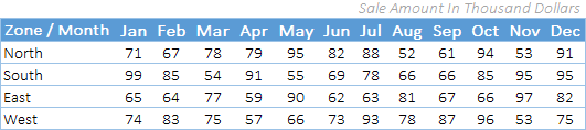
Below is an example of a simple heat map where we have zone-wise and month-wise data and for every cell where we have sales value there is color shade applied on the cell.


And this color shade helps us to quickly compare values in the cells with each other. Cell with the highest value has green color as the cell color and the cell with the lowest value has red, and all the cell in the middle has a yellow color.
All the values between the highest value and the lowest value have color shade according to their rank. But you can create a heat map like this manually because applying a color to a cell according to its values can be possible every time.
Now the point is, you how you can what are the possible ways to create a heat map in Excel. And, if you ask me there are more than three. So in this post, I’ll be sharing all the possible ways to create a heat map in Excel.
When you take a printout of a heat map on paper it looks really nasty especially when you are using a black and white printer. All the shades only have black and white color which is not easy to understand for anyone.
Create a Heat Map in Excel using Conditional Formatting
If you don’t want to put extra effort and save your time then you can create a simple heat map by using conditional formatting. I’m using the same data as a sample (DOWNLOAD LINK) here which I have shown you at the starting of this post.

To create a heat map in Excel you need to follow the below steps:
- First of all, select the data on which you want to apply a heat map (here you need to select all the cells where you have sales values)
- After that, go to Home Tab ➜ Styles ➜ Conditional Formatting.
- In conditional formatting options, selects color scales. (You have six different types of color scales to choose from).

- Once you select an option, all the cells will get a color shade according to the value which they have and you’ll get a heat map like below.

- And, if you want to hide value and only want to show color shared you can use custom formatting for this.
- For this, first of all, select heat map data and open formatting options (Ctrl + 1).
- Now, in the number tab, go to custom and enter ;;; and in the end click OK.

- Once you click OK, all the number will be hide from the cells. Well, hey are in the cells but just hidden.


Steps to add a Heat Map in a Pivot Table
You can also use heat in a pivot table by applying conditional formatting. These are the steps to follow:
- Select any of the cells in the pivot table.
- Go to Home Tab ➜ Styles ➜ Conditional Formatting.
- In conditional formatting options, selects color scales.


Further, if you want to hide numbers (which I don’t recommend) please follow these simple steps.
- Select any of the cells in the pivot table.
- Go To Analyze Tab ➜ Active Field ➜ Field Settings.

- Click on number format.
- In number tab, go to custom and enter ;;; in type.
- Click OK.

You can download this sample file from here to learn how we can use a slicer with a heat map pivot.
Steps to Create a Dynamic Heat Map in Excel
You can create a dynamic heat map if you want to hide/show it according to your need.

Below is the table we have used to create a dynamic heat map.

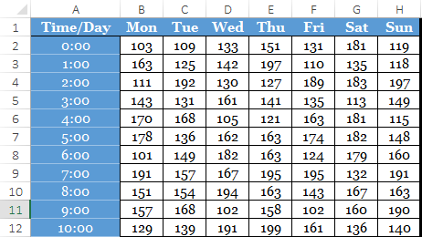
And following things we need to incorporate.
- Option to switch between heat-map and numbers.
- Auto update table with heat map when add new data.
Here’s how to do this:

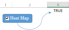
Now you have a dynamic heat map that you can control with a check box.

And if you want to hide numbers when you tick the marked checkbox you need to create a separate conditional formatting rule. Here’s how to do this:
- Open conditional formatting new rule dialog box.
- Select “Use a formula to select which cell to format” and enter the below formula.

- =IF($K$1=TRUE,TRUE,FALSE)
- Now, specify custom number formatting.

After applying all the above customization you will get a dynamic heat map.
More Information
These ate some links to help you out while choosing your favorite color scheme.
Sample File
Download this sample from here to learn more.
Conclusion
Imagine if you are looking at a large data set, it’s really hard to identify the lower values or higher values, but if you have a heat map then it’s easy to identify them.
You can use different color schemes to illustrate a heat map. And, if you can put some extra effort then a dynamic heat map is the best. I hope this tips will help you to get better at Excel and now tell one thing.
Do you think a heat map can be helpful for you in your work?
Share your views with me in the comment section, I’d love to hear from you. And, please don’t forget to share this tip with your friends.